Machine learning practice 3

(a)

Create a binary variable that takes on a 1 for cars with gas mileage above the median, and a 0 for cars with gas mileage below the median.

Answer:

df <- Auto %>%
  mutate(mpg01=ifelse(mpg > median(mpg), 1, 0) %>% as.factor) %>%
  select(-c(mpg, name))

(b)

Fit a support vector classifier to the data with various values of cost, in order to predict whether a car gets high or low gas mileage. Report the cross-validation errors associated with different values of this parameter. Comment on your results.

Answer:

set.seed(1996)
linear_tune <- tune(svm, mpg01 ~ ., data = df, kernel = "linear",
                 ranges = list(cost = c(.001, .01, .1, 1, 5, 10, 100)))
summary(linear_tune)
linear_tune$best.parameters
linear_tune$best.performance

Results presents that cross-validation error was minimized when cost equals 5.

(c)

Now repeat (b), this time using SVMs with radial and polynomial basis kernels, with different values of gamma and degree and cost. Comment on your results.

Answer:

radial basis kernels:

set.seed(1996)
radial_tune <- tune(svm, mpg01~., data=df, kernel='radial',
                 ranges = list(cost = c(.001, .01, .1, 1, 5, 10, 100,1000),
                               gamma = c(0.5, 1, 2, 3, 4)))
radial_tune$best.parameters
radial_tune$best.performance

As we can see from the output, the training CV error is minimized for a radial model at cost=1 and gamma=1. In addition, the training CV error is a little better than that of the linear kernel model.

polynomial basis kernels:

set.seed(1996)
poly_tune = tune(svm, mpg01~., data=df, kernel='polynomial',
                 ranges = list(cost = c(.001, .01, .1, 1, 5, 10, 100,1000),
                               degree = c(1,2,3,4,5)))
poly_tune$best.parameters
poly_tune$best.performance

As we can see from the output, the training CV error is minimized for a polynomial model at cost=5 and degree=3, which suggested the true decision boundary is non-linear. In addition, the training CV error is better than that of the linear kernel model but worse than that of the radial kernel model.

(d)

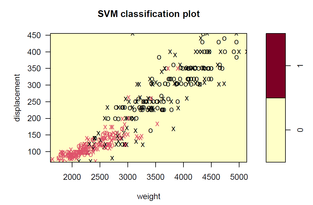
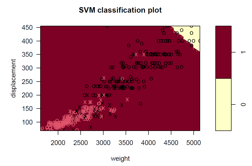
Make some plots to back up your assertions in (b) and (c).

svmfit_l <- svm(mpg01~., data=df, kernel="linear", cost=5)
svmfit_r <- svm(mpg01~., data=df, kernel="radial", cost=1, gamma=1)
svmfit_p <- svm(mpg01~., data=df, kernel="polynomial", cost=5, degree=3)
names_list <- names(df)[-8]

# some plots

#linear
plot(svmfit_l, df, displacement~weight)

#radial
plot(svmfit_r, df, displacement~weight)

#polynomial
plot(svmfit_p, df, displacement~weight)

(a)

Run \(K\)-means for \(K\) from 1 to 20 and plot the associated within cluster sum of squares (WSSs). Comment the WSS at \(K=3\).

wss <- NULL
for(i in 1:20){
  kmeansfit <- kmeans(Gene, centers = i, nstart = 20)
  temp <- data.frame(value=kmeansfit$betweenss/kmeansfit$totss,
                     clusters=i)
  wss <- rbind(wss, temp)
}
plot(wss$clusters, wss$value, type="b", 
     xlab = "number of clusters", ylab = "WSS value")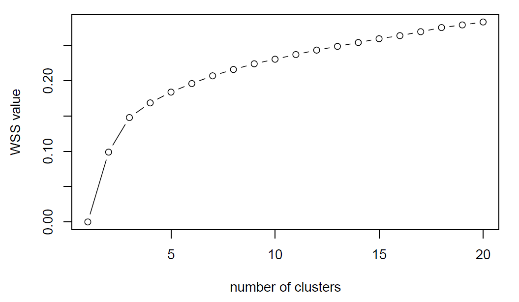

k3 <- kmeans(Gene, centers = 3, nstart = 20)
k3$betweenss/k3$totss

Comment the WSS at \(K=3\): The 14.8% is a measure of the total variance in our data set that is explained by the clustering. k-means minimize the within group dispersion and maximize the between-group dispersion. By assigning the samples to 3 clusters rather than 563 (number of samples) clusters achieved a reduction in sums of squares of 14.8%.

(b)

Apply \(K\)-means with \(K=3\) to the Gene dataset. What percentage of Basal, LumA, and LumB type samples are in each of the 3 resulting clusters? Did we do a good job distinguishing LumA from LumB? Confusion matrix of clusters versus subtypes might be helpful.

results <- data.frame(Subtypes,pred=k3$cluster) %>% filter(Subtypes!="Basal")
table(results$Subtypes,results$pred)

According to the simple counting table, we found that LumA should be matching with 2 and LumB should be matching with 1. Then we can have confusion matrix of clusters versus subtypes,

tibble(LumA = c(192, 117),
       LumB = c(27, 125),
       pred = c("LumA (pred)", "LumB (pred)")) %>% 
  column_to_rownames(var = "pred")
(192+125)/(461)

As we can tell from the confusion matrix that the overall classify accuracy is 68.8%, which is satisfying.

(c)

Now apply PCA to the Gene dataset. Plot the data in the first two PCs colored by Subtypes. Does this plot appear to separate the cancer subtypes well?

Gene_df <- Gene[, colSums(Gene == 0) != nrow(Gene)]
# Dimension reduction using PCA
res.pca <- prcomp(Gene_df,  scale = TRUE)
#Visualize eigenvalues (scree plot).
fviz_eig(res.pca)
#Graph of individuals.
fviz_pca_ind(res.pca,
             col.ind = as.factor(Subtypes), # color by groups
             palette = c("#00AFBB", "#E7B800", "#FC4E07"),
             legend.title = "Groups",
             repel = TRUE
             )

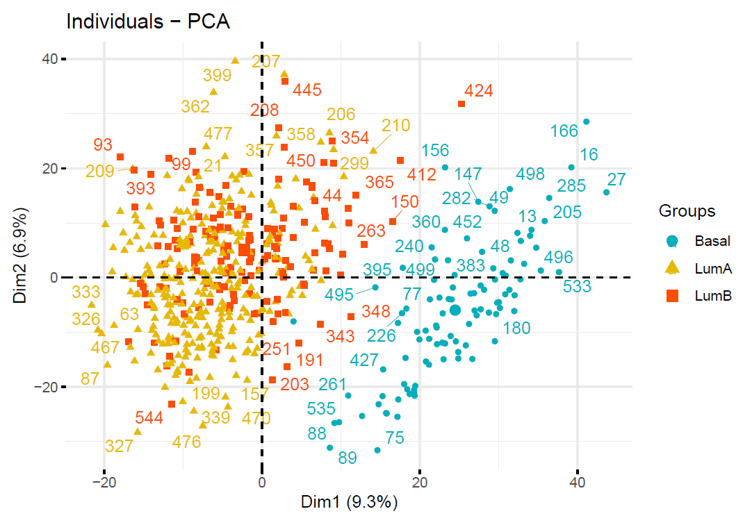As we can tell from the plot, PCA appears to separate the cancer subtypes well.

(d)

Try plotting some more PC combinations. Can you find a pair of PCs that appear to separate all three subtypes well? Report the scatterplot of the data for pair of PCs that you think best separates all three types.

# Coordinates of individuals
ind.coord <- data.frame(type=as.factor(Subtypes), get_pca_ind(res.pca)$coord)

index <- 1
for(i in 1:5){
  for(k in (i+1):6){
    ggplot(ind.coord) +
      geom_point(aes_string(x=names(ind.coord)[i+1], y=names(ind.coord)[k+1], 
                            color="type"))+theme_bw() -> temp
    assign(paste0("p_",index), temp)
    index <- index+1
  }
}
ggarrange(plotlist=mget(paste0("p_",c(1:6))), 
          nrow = 3, ncol = 2)
ggarrange(plotlist=mget(paste0("p_",c(7:12))), 
          nrow = 3, ncol = 2)
ggarrange(plotlist=mget(paste0("p_",c(13:15))), 
          nrow = 3, ncol = 1)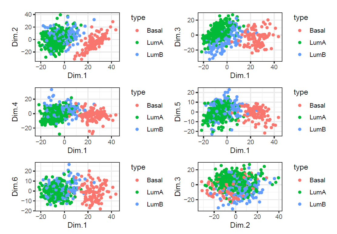

According to plots, we cannot find a pair of PCs that appear to separate all three subtypes well. The best pair of PCs that separates all three types is Dim1&PCDim3.

(e)

Perform \(K\)-means with \(K=3\) on the pair of PCs identified in (d). Report the confusion matrix and make some comments.

k3 <- kmeans(ind.coord[,c(2,4)], centers = 3, nstart = 20)
results <- data.frame(Subtypes,pred=k3$cluster)
table(results$Subtypes,results$pred)

According to the simple counting table, we found that LumA should be matching with 2 and LumB should be matching with 3. Then we can have confusion matrix of clusters versus subtypes,

tibble(Basal = c(101, 1, 0),
       LumA = c(0, 201, 108),
       LumB = c(10, 41, 101),
       pred = c("Basal (pred)", "LumA (pred)", "LumB (pred)")) %>% 
  column_to_rownames(var = "pred")
(201+101)/(201+108+41+101)

As we can tell from the confusion matrix for LumA and LumB that the overall classify accuracy is 67.0%, which is largely consistent with the results when we applied \(K\)-means with \(K=3\) algorithm directly.

(f)

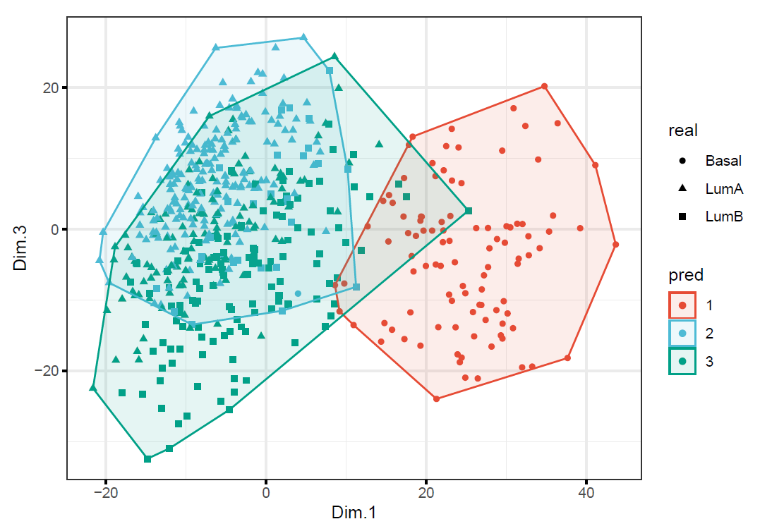
Create two plots colored by the clusters found in (b) and in (e) respectively. Do they look similarly or differently? Explain why using PCA to reduce the number of dimensions from 2000 to 2 did not significantly change the results of \(K\)-means.

k3_origin <- kmeans(Gene_df, centers = 3, nstart = 20)
# clusters found in (b)
data.frame(real=as.factor(Subtypes), 
           pred=as.factor(k3_origin$cluster),ind.coord)%>%
  ggscatter(
  ., x = "Dim.1", y = "Dim.3", 
  color = "pred", palette = "npg", ellipse = TRUE, ellipse.type = "convex",
  shape = "real", size = 1.5,  legend = "right", ggtheme = theme_bw()
)

# clusters found in (e)
data.frame(real=as.factor(Subtypes), 
           pred=as.factor(k3$cluster),ind.coord)%>%
  ggscatter(
  ., x = "Dim.1", y = "Dim.3", 
  color = "pred", palette = "npg", ellipse = TRUE, ellipse.type = "convex",
  shape = "real", size = 1.5,  legend = "right", ggtheme = theme_bw()
)

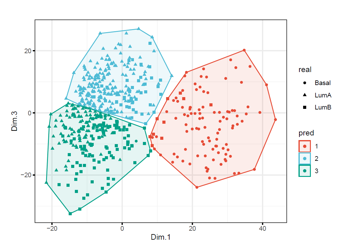
As we can tell from the plots that two model provided different clusters (but similar classification accuracy). Research (Yeung & Ruzzo, 2000) showed that clustering with the PC’s rather than the original dims does not necessarily improve cluster quality. In this question, since none of PC’s (which contain most of the variation in the data) capture the cluster structure well, it cannot improve the classification accuracy.

(g)

Now apply MDS with various metrics and non-metric MDS to Gene to obtain 2-dimensional representations. Does any of them provide better separated scatterplot as compared to that from (d)? Notice that the Euclidean metric in MDS gives the same representation as PCA does.

# Compute classic MDS
mds_c <- Gene %>%
  dist() %>%          
  cmdscale(k = 2) %>%
  as_tibble() %>%
  mutate(type=as.factor(Subtypes))
colnames(mds_c)[1:2] <- c("Dim.1", "Dim.2")
# Plot MDS
ggplot(mds_c) +
  geom_point(aes(x=Dim.1, y=Dim.2, color=type)) + theme_bw()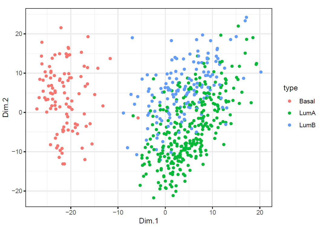

# Compute non-metric MDS
mds_n <- Gene %>%
  dist() %>%          
  isoMDS(k = 2) %>%
  .$points %>%
  as_tibble() %>%
  mutate(type=as.factor(Subtypes))
colnames(mds_n)[1:2] <- c("Dim.1", "Dim.2")
# Plot MDS
ggplot(mds_n) +
  geom_point(aes(x=Dim.1, y=Dim.2, color=type)) + theme_bw()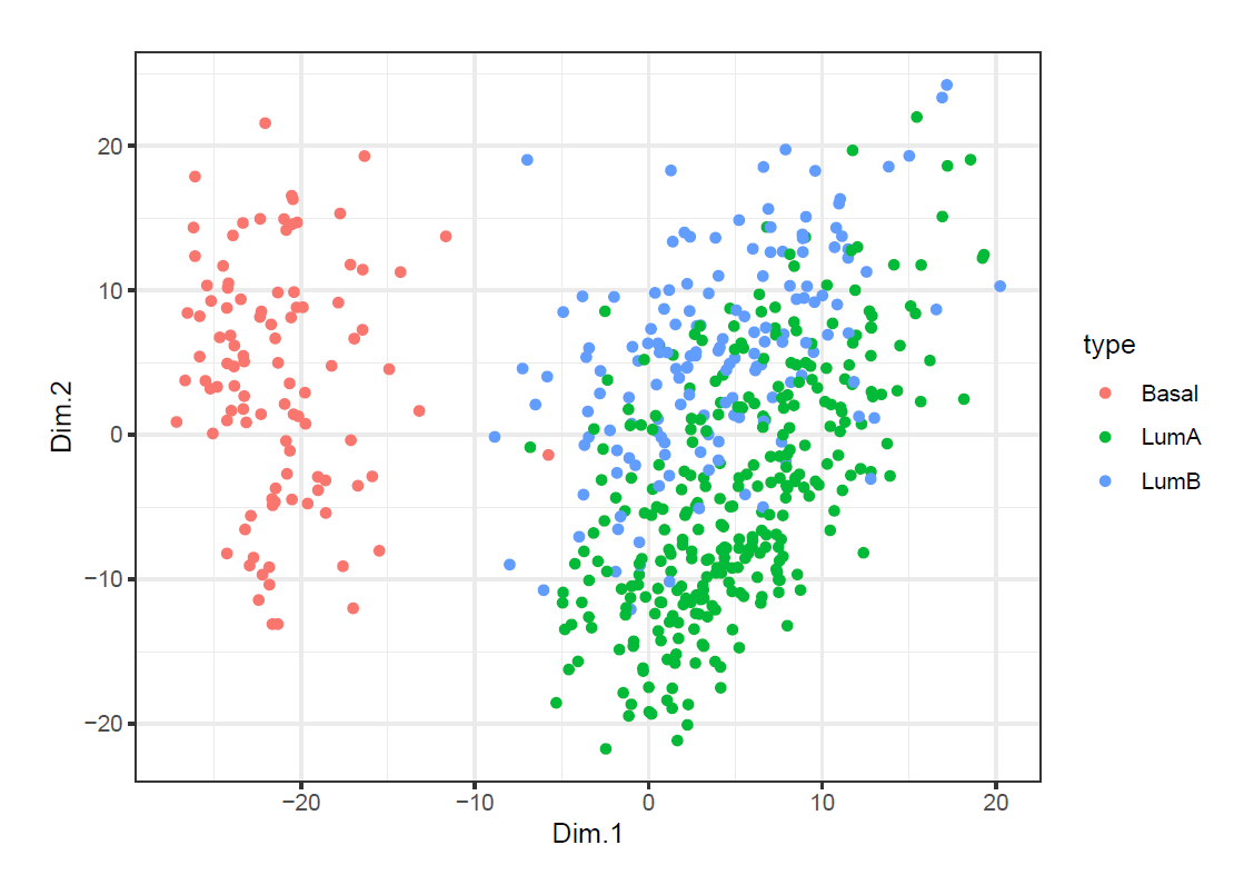

We can tell from the plots that both of them provide similar separated scatterplot as compared to that from (d).

(h)

Perform \(K\)-means with \(K=3\) on the new representations from (g) and report the confusion matrices. Compare them with that from (e).

k3_mdsc <- kmeans(mds_c[,1:2], centers = 3, nstart = 20)
results <- data.frame(Subtypes,pred=k3_mdsc$cluster)
table(results$Subtypes,results$pred)

k3_mdsn <- kmeans(mds_n[,1:2], centers = 3, nstart = 20)
results <- data.frame(Subtypes,pred=k3_mdsn$cluster)
table(results$Subtypes,results$pred)

According to the simple counting table, we found that classic mds and non-metric mds provides same results. Then we can have confusion matrix of clusters versus subtypes,

tibble(LumA = c(195, 114),
       LumB = c(33, 117),
       pred = c( "LumA (pred)", "LumB (pred)")) %>% 
  column_to_rownames(var = "pred")
(195+117)/(195+114+33+117)

As we can tell from the confusion matrix for LumA and LumB that the overall classify accuracy is 68.0%, which is very close to the results we obtained in (e).

(i)

Suppose we might know that the first PC contains information we aren’t interested in. Apply \(K\)-means with \(K=3\) to Gene dataset subtracting the approximation from the first PC. Report the confusion matrix and make some comments.

k3 <- kmeans(ind.coord[,-c(1:2)], centers = 3, nstart = 20)
results <- data.frame(Subtypes,pred=k3$cluster)
table(results$Subtypes,results$pred)

According to the simple counting table, we found that classic mds and non-metric mds provides same results. Then we can have confusion matrix of clusters versus subtypes,

tibble(LumA = c(140, 61),
       LumB = c(19, 94),
       pred = c( "LumA (pred)", "LumB (pred)")) %>% 
  column_to_rownames(var = "pred")
(140+94)/(140+61+19+94)

As we can tell from the confusion matrix for LumA and LumB that the overall classify accuracy is 74.5%, which is better than the model including the first PC. But 106 LumA and 39 LumB cases are wrongly classified as Basal, which is much worse than the model including the first PC (\(\leq10\) LumA and \(\leq10\) LumB).