Machine learning practice 2

(a)

Create a binary variable, mpg01, that contains a 1 if mpg contains a value above its median, and a 0 if mpg contains a value below its median.

Answer:

df <- Auto %>%
  mutate(mpg01=ifelse(mpg > median(mpg), 1, 0) %>% as.factor)

(b)

Explore the data graphically in order to investigate the association between mgp01 and the other features. Which of the other features seem most likely to be useful in predicting mpg01? Scatterplots and boxplots may be useful tools to answer this question. Describe your findings.

Answer:

df %>% 
  mutate(name_unclass = unclass(name)) %>%
  mutate_at(vars(names(df)[c(2,8)]),as.factor)-> df_p
vars_need <- dput(names(df_p))[-c(1,9,10)]
for(i in 1:8){
  if(i %in% c(1,7)){
    ggplot(df_p, aes_string(x=vars_need[i], y="mpg", fill="mpg01")) +
      geom_boxplot() +
      theme_bw() +
      theme(legend.position = "none") -> temp
  }else{
    ggplot(df_p, aes_string(vars_need[i], "mpg", group="mpg01", color="mpg01")) + 
      geom_point() + 
      xlab(vars_need[i]) +
      scale_color_manual(values = c('#999999','#E69F00')) + 
      #geom_smooth(method=lm, se=T, fullrange=T)+
      theme_bw()+
      theme(legend.position = "none")-> temp
  }
  temp_name <- paste0("fig_",i)
  assign(temp_name, temp)
}

ggarrange(plotlist=mget(paste0("fig_",c(1:8))), 
          nrow = 3, ncol = 3, labels = 1:8)

According to the scatter plot and boxplot, we found that variable displacement, horsepower, weight, acceleration and year are most likely to be useful in predicting mpg01.

(c)

Split the data into a training set and a test set with ratio 2:1.

Answer:

set.seed(1996)
trainid <- sample(1:nrow(df), nrow(df)*2/3 %>% round, replace=F) 
train <- df[trainid,]
test <- df[-trainid,]

(d)

Perform LDA on the training data in order to predict mpg01 using the variables that seemed most associated with mpg01 in (b). What is the test error of the model obtained?

Answer:

ldafit <- lda(mpg01 ~ displacement+horsepower+weight+acceleration+year, 
               data=train)
ldafit_pred <- predict(ldafit, test)$class
table(ldafit_pred, test$mpg01)

# test error
mean(ldafit_pred != test$mpg01)

test error rate: 9.92%

(e)

Perform QDA on the training data in order to predict mpg01 using the variables that seemed most associated with mpg01 in (b). What is the test error of the model obtained?

Answer:

qdafit <- qda(mpg01 ~ displacement+horsepower+weight+acceleration+year, 
               data=train)
qdafit_pred <- predict(qdafit, test)$class
table(qdafit_pred, test$mpg01)

# test error
mean(qdafit_pred != test$mpg01)

test error rate: 10.69%

(f)

Perform logistic regression on the training data in order to predict mpg01 using the variables that seemed most associated with mpg01 in (b). What is the test error of the model obtained?

Answer:

logitfit <- glm(mpg01 ~ displacement+horsepower+weight+acceleration+year, 
                data=train, family=binomial)
logitfit_prob <- predict(logitfit, test, type="response")
logitfit_pred <- ifelse(logitfit_prob > 0.5, 1, 0)
table(logitfit_pred, test$mpg01)

# error rate
mean(logitfit_pred != test$mpg01)  

test error rate is 10.69%, which turned out to be the same as that of QDA.

(a)

Use the poly() function to fit a cubic polynomial regression to predict nox using dis. Report the regression output, and plot the data and resulting polynomial fits.

Answer:

lmfit = lm(nox ~ poly(dis, 3), data = Boston)
summary(lmfit)

dislims <- range(Boston$dis)
dis.grid <- seq(dislims[1], dislims[2], 0.1)
preds <- predict(lmfit, newdata=list(dis=dis.grid), se=TRUE)
se95 <- preds$fit + cbind(1.96*preds$se.fit, -1.96*preds$se.fit)
plot(Boston$dis, Boston$nox, xlim=dislims, cex=0.5)
lines(dis.grid, preds$fit, lwd=2.5, col="blue")
matlines(dis.grid, se95, lwd=1.5, col="blue", lty=2)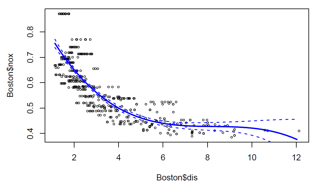

(b)

Plot the polynomial fits for a range of different polynomial degrees (say, from 1 to 10), and report the associated residual sum of squares.

Answer:

rss.error <- NULL
for (i in 1:10) {
  lmfit <- lm(nox ~ poly(dis,i), data=Boston)
  rss.error <- rbind(rss.error, 
                     data.frame(rss.error=sum(lmfit$residuals^2),
                                polynomial.degrees=i))
}

# report the associated residual sum of squares
rss.error
plot(rss.error$polynomial.degrees, rss.error$rss.error, type="b")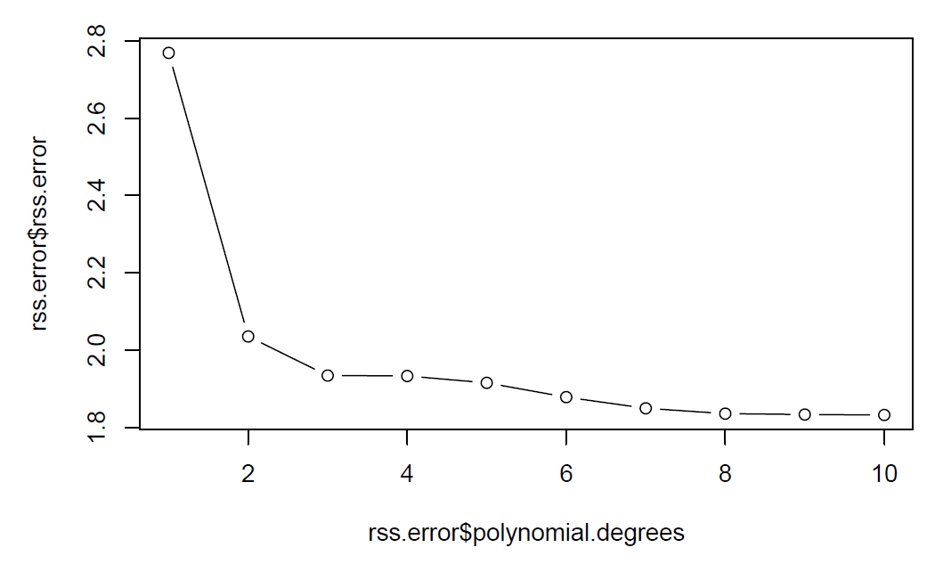

We can tell from the plot that rss decreases monotonically when polynomial degrees increase.

(c)

Perform cross-validation to select the optimal degree for the polynomial, and explain your results.

Answer:

cv.error <- NULL
for (i in 1:10) {
  set.seed(1996)
  glm.fit <- glm(nox~poly(dis,i), family = gaussian, data=Boston)
  temp <- cv.glm(Boston, glm.fit, K=10)$delta[2]
  cv.error <- rbind(cv.error, 
                    data.frame(rss.error=temp, polynomial.degrees=i))
}
cv.error
plot(cv.error$polynomial.degrees, cv.error$rss.error, type="b")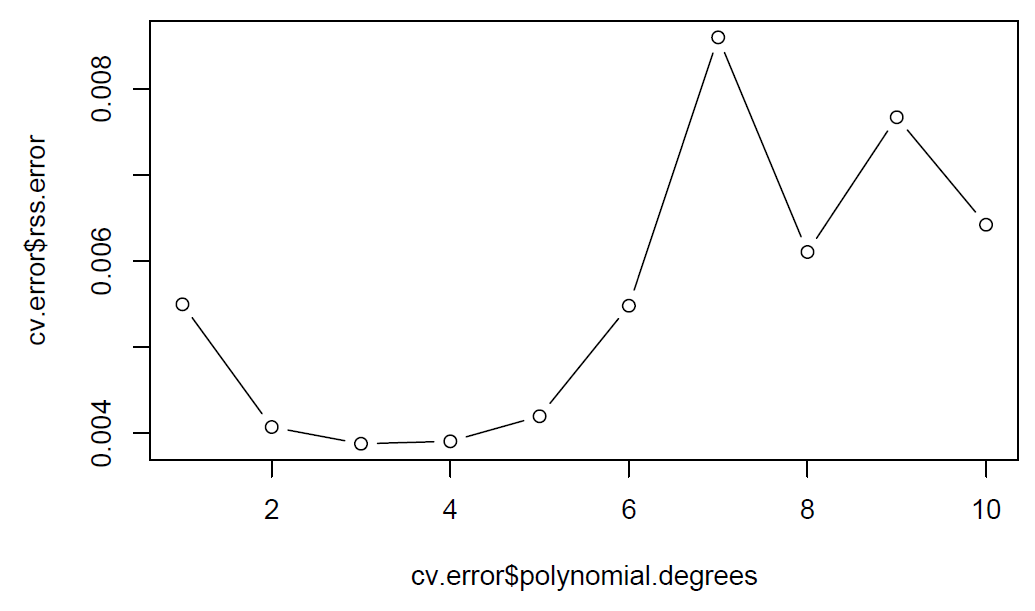

According to the plot, we see that the CV error reduces when polynomial degrees increase from 1 to 3 and does not show clear improvement after degree 3 polynomial. Thus, we pick 3 as the best polynomial degree.

(d)

Use the bs() function to fit a regression spline to predict nox using dis. Report the output for the fit using four degrees of freedom. How did you choose the knots? Plot the resulting fit.

Answer:

We choose the knots as the 25%, 50% and 75% quantile of the dis data.

knots_set <- summary(Boston$dis) %>% as.numeric %>% .[c(2,3,5)]
spfit <- lm(nox ~ bs(dis, df = 4, knots = knots_set), data = Boston)

#Report the model summary
summary(spfit)

#Resulting fit
sppred <- predict(spfit, list(dis = dis.grid))
plot(nox ~ dis, data = Boston)
lines(dis.grid, sppred, col = "blue", lwd = 2)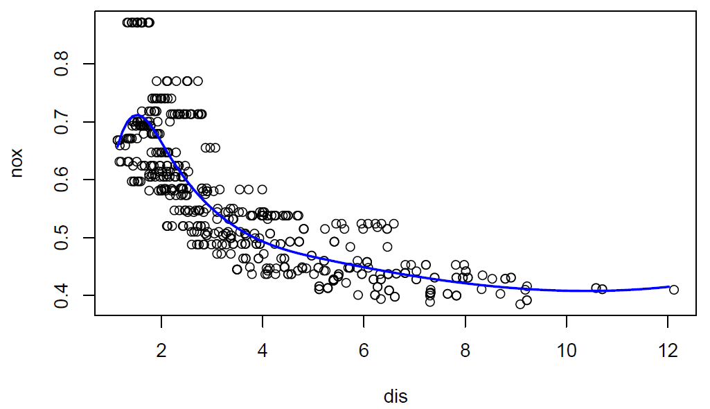

The prediction line seems to fit the data well.

(e)

Now fit a regression spline for a range of degrees of freedom, and plot the resulting fits and report the resulting RSS. Describe the results obtained.

Answer:

rss.error <- NULL
for (i in 4:16) {
  spfit <- lm(nox~bs(dis, df=i), data=Boston)
  rss.error <- rbind(rss.error, 
                     data.frame(rss.error=sum(spfit$residuals^2),
                                polynomial.degrees=i))
}

# report the associated residual sum of squares
rss.error
plot(rss.error$polynomial.degrees, rss.error$rss.error, type="b")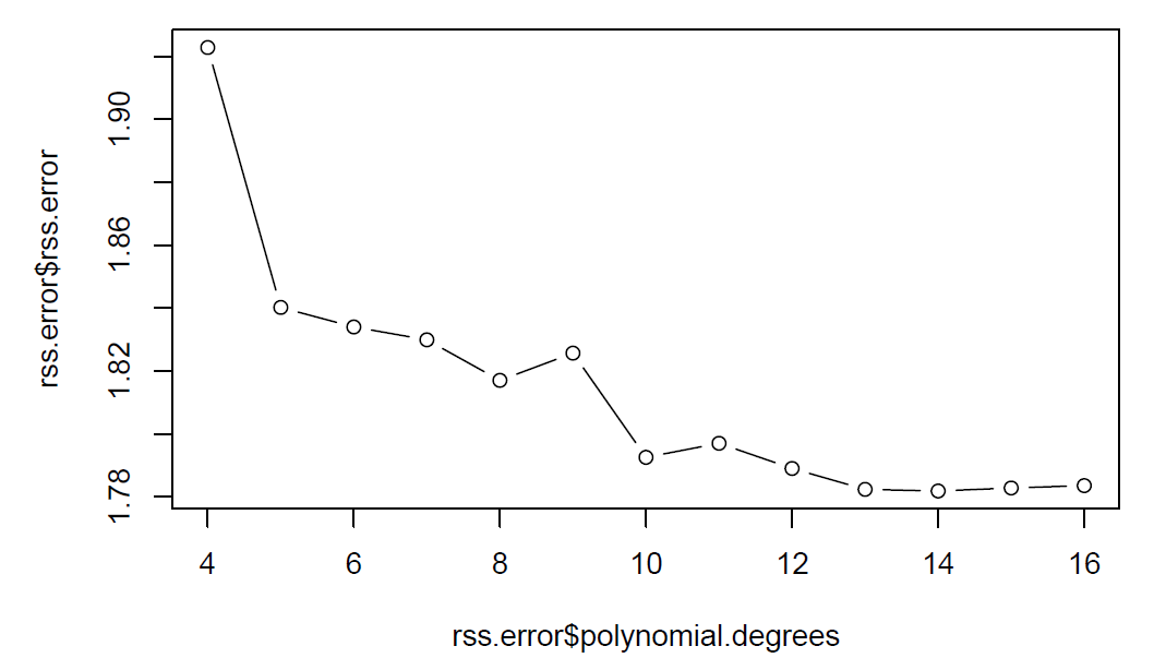

We can tell from the plots that rss error reduces when degrees of freedom increase from 4 to 14 and does not show clear improvement after 14 degrees of freedom.

(f)

Perform cross-validation to select the best degrees of freedom for a regression spline on this data. Describe your results.

Answer:

cv.error <- NULL
for (i in 4:16) {
  set.seed(19969)
  glm.fit <- glm(nox ~ bs(dis, df = i), family = gaussian, data=Boston)
  temp <- cv.glm(Boston, glm.fit, K=10)$delta[2] # adjusted cross-validation estimate
  cv.error <- rbind(cv.error, 
                    data.frame(rss.error=temp, polynomial.degrees=i))
}
cv.error
plot(cv.error$polynomial.degrees, cv.error$rss.error, type="b")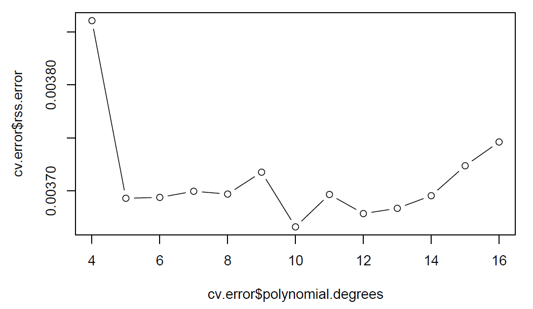

After 10-folds cross-validation, we can tell from the plots that cv error reach the minimum value at 10 degrees of freedom and does not show clear improvement after 10 degrees of freedom. Thus, we choose 10 as the best degrees of freedom.