Machine learning practice 1
- (Model Selection, [ISL] 6.8, 25 pt) In this exercise, we will generate simulated data, and will then use this data to perform model selection.
- Use the
rnormfunction to generate a predictor \(X\) of length \(n = 100\), as well as a noise vector \(\epsilon\) of length \(n = 100\).
set.seed(199609)
X <- rnorm(100)
epsilon <- rnorm(100)- Generate a response vector \(Y\) of length \(n = 100\) according to the model \[ Y = \beta_0 + \beta_1 X + \beta_2 X^2 + \beta_3 X^3 + \epsilon, \] where \(\beta_0 = 3\), \(\beta_1 = 2\), \(\beta_2 = -3\), \(\beta_3 = 0.3\).
b0 <- 3 ; b1 <- 2 ; b2 <- -3 ; b3 <- 0.3

Y <- b0 + b1*X + b2*X^2 + b3*X^3 + epsilon- Use the
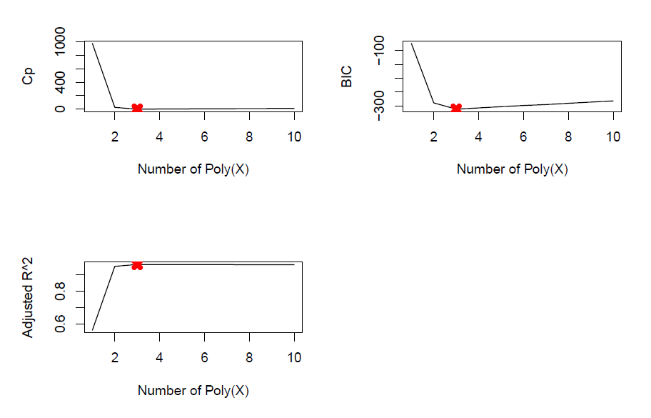
regsubsetsfunction fromleapspackage to perform best subset selection in order to choose the best model from the set of predictors \((X, X^2, \cdots, X^{10})\). What are the best models obtained according to \(C_p\), BIC, and adjusted \(R^2\), respectively? Show some plots to provide evidence for your answer, and report the coefficients of the best model obtained.
df <- data.frame(X,X^2,X^3,X^4,X^5,X^6,X^7,X^8,X^9,X^10,Y)
best_model <- regsubsets(Y ~ ., data = df, nvmax=10)
summary_model <- best_model %>% summary

#the best models according to C_p, BIC, and adjusted R^2
min.cp <- which.min(summary_model$cp)
min.cp
min.bic <- which.min(summary_model$bic)
min.bic
min.adjr2 <- which.max(summary_model$adjr2)
min.adjr2

# plots that show the best models
par(mfrow = c(2,2))
plot(summary_model$cp, xlab = "Number of Poly(X)",
     ylab ="Cp", type="l")
points(min.cp, summary_model$cp[min.cp], col = "red", pch = 4, lwd = 5)

plot(summary_model$bic, xlab = "Number of Poly(X)",
     ylab = "BIC", type="l")
points(min.bic, summary_model$bic[min.bic], col = "red", pch = 4, lwd = 5)

plot(summary_model$adjr2, xlab = "Number of Poly(X)",
     ylab = "Adjusted R^2", type="l")
points(min.adjr2, summary_model$adjr2[min.adjr2], col = "red", pch = 4, lwd = 5)

coef(best_model, min.cp)
coef(best_model, min.bic)
coef(best_model, min.adjr2)
- Repeat (c), using forward stepwise selection and also using backward stepwise selection. How does your answer compare to the results in (c)?
# forward stepwise selection.
best_model_f <- regsubsets(Y~., data=df, nvmax=10, method='forward')
summary_model_f <- best_model_f %>% summary

# refer to C_p, BIC, and adjusted R^2
min.cp <- which.min(summary_model_f$cp)
min.cp
min.bic <- which.min(summary_model_f$bic)
min.bic
min.adjr2 <- which.max(summary_model_f$adjr2)
min.adjr2

coef(best_model, min.cp)
coef(best_model, min.bic)
coef(best_model, min.adjr2)

# backward stepwise selection.
best_model_b = regsubsets(Y~., data=df, nvmax=10, method='backward')
summary_model_b <- best_model_f %>% summary

#the best models according to C_p, BIC, and adjusted R^2
min.cp <- which.min(summary_model_b$cp)
min.cp
min.bic <- which.min(summary_model_b$bic)
min.bic
min.adjr2 <- which.max(summary_model_b$adjr2)
min.adjr2

coef(best_model, min.cp)
coef(best_model, min.bic)
coef(best_model, min.adjr2)
We found that both forward and backward method provided same results as part (c).
- Now fit a LASSO model with
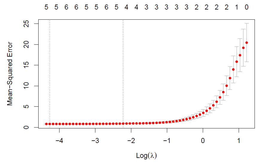
glmnetfunction fromglmnetpackage to the simulated data, again using \((X,X^2,\cdots,X^{10})\) as predictors. Use cross-validation to select the optimal value of \(\lambda\). Create plots of the cross-validation error as a function of \(\lambda\). Report the resulting coefficient estimates, and discuss the results obtained.
# Lasso model
lasso = glmnet(df[, -11]%>%as.matrix, df[, 11], alpha=1)
# cross-validation
cv.out = cv.glmnet(df[, -11]%>%as.matrix, df[, 11], alpha=1)
# cross-validation error
plot(cv.out)
# the optimal value of lambda
best_lam = cv.out$lambda.min
# Coefficients from lasso model with best lambda.
predict(lasso, s=best_lam, type="coefficients")
According the results, we see that estimated coefficients of b1~b3 from lasso model with best lambda are largely consistent with the true value of b1~b3. Nevertheless, lasso model included X^7 and X^9 by mistake, with small coefficients.
- Now generate a response vector \(Y\) according to the model \[Y = \beta_0 + \beta_7 X^7 + \epsilon,\] where \(\beta_7 = 7\), and perform best subset selection and the LASSO. Discuss the results obtained.
# generate y2
b7 <- 7
Y2 <- b0 + b7*X^7 + epsilon

df <- data.frame(X,X^2,X^3,X^4,X^5,X^6,X^7,X^8,X^9,X^10,Y2)

# best subset selection
best_model <- regsubsets(Y2 ~ ., data=df, nvmax=10)
summary_model <- summary(best_model)

# refer to C_p, BIC, and adjusted R^2
min.cp <- which.min(summary_model$cp)
min.bic <- which.min(summary_model$bic)
min.adjr2 <- which.max(summary_model$adjr2)

# check results
coef(best_model, min.cp)
coef(best_model, min.bic)
coef(best_model, min.adjr2)

# LASSO model
lasso = glmnet(df[, -11]%>%as.matrix, df[, 11], alpha=1)
# cross-validation
cv.out = cv.glmnet(df[, -11]%>%as.matrix, df[, 11], alpha=1)
# cross-validation error
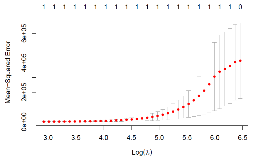
plot(cv.out)
# the optimal value of lambda
best_lam = cv.out$lambda.min
# Coefficients from lasso model with best lambda.
predict(lasso, s=best_lam, type="coefficients")
According to the results, we found that the best subset selection (referring to the BIC value) and Lasso regression provides the relatively more accurate estimates than that of best subset selection (referring to C_p and adjusted R^2).
- (Prediction, [ISL] 6.9, 20 pt) In this exercise, we will predict the number of applications received (
Apps) using the other variables in theCollegedata set fromISLRpackage.
- Randomly split the data set into equal sized training set and test set (1:1).
data(College)

set.seed(199609)
train_id <- sample(dim(College)[1], dim(College)[1]/2)

train_set <- College[train_id, ]
test_set <- College[-train_id, ]- Fit a linear model using least squares on the training set, and report the test error obtained.
# linear model
modl <- lm(Apps~., data = train_set)
summary(modl)
pred1 <- predict(modl, newdata = test_set[,-2], type = "response")

# test error
MAE(pred1, College$Apps[-train_id])
MSE(pred1, College$Apps[-train_id])
RMSE(pred1, College$Apps[-train_id])
R2(pred1, College$Apps[-train_id], form = "traditional")

err1 <- data.frame(MAE = MAE(pred1, College$Apps[-train_id]),
                  MSE = MSE(pred1, College$Apps[-train_id]),
                  RMSE = RMSE(pred1, College$Apps[-train_id]),
R2 = R2(pred1, College$Apps[-train_id], form = "traditional"))- Fit a ridge regression model on the training set, with \(\lambda\) chosen by 5-fold cross-validation. Report the test error obtained.
# prepare data
train_set <- model.matrix(Apps~.-1, data=College[train_id, ])
test_set <- model.matrix(Apps~.-1, data=College[-train_id, ])

# ridge regression with cross-validation
modr_cv <- cv.glmnet(train_set %>% as.matrix,
                     College$Apps[train_id] %>% as.matrix,
                     nfolds = 5, alpha = 0)
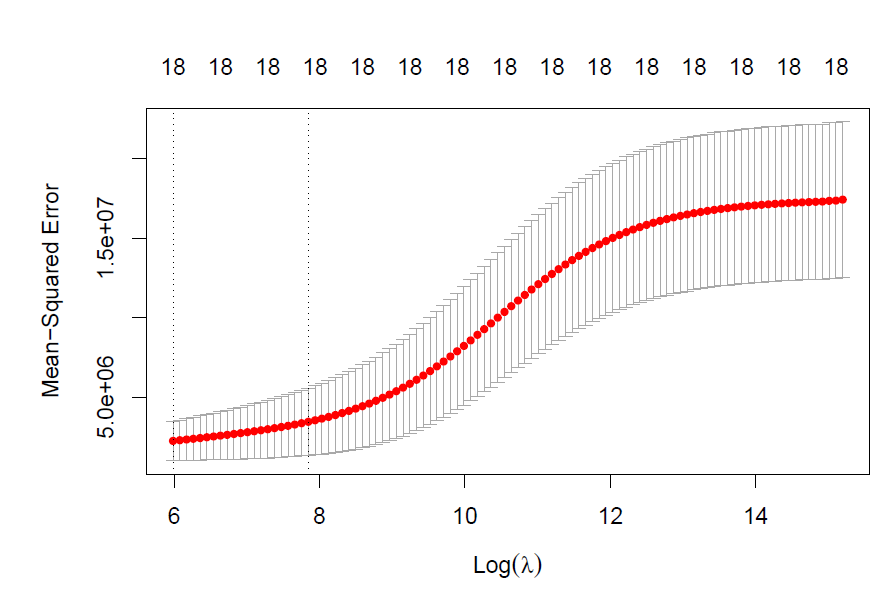
plot(modr_cv)
lambda <- modr_cv$lambda.min
pred2 <- predict(modr_cv, s = lambda, newx = test_set)
summary(modr_cv)
# test error
MAE(pred2, College$Apps[-train_id])
MSE(pred2, College$Apps[-train_id])
RMSE(pred2, College$Apps[-train_id])
R2(pred2, College$Apps[-train_id], form = "traditional")

err2 <- data.frame(MAE = MAE(pred2, College$Apps[-train_id]),
                  MSE = MSE(pred2, College$Apps[-train_id]),
                  RMSE = RMSE(pred2, College$Apps[-train_id]),
                  R2 = R2(pred2, College$Apps[-train_id], form = "traditional"))
- Fit a LASSO model on the training set, with \(\lambda\) chosen by 5-fold cross-validation. Report the test error obtained, along with the number of non-zero coefficient estimates.
# LASSO regression with cross-validation
modr_cv <- cv.glmnet(train_set %>% as.matrix,
                     College$Apps[train_id] %>% as.matrix,
                     nfolds = 5, alpha = 1)
plot(modr_cv)
lambda <- modr_cv$lambda.min
pred3 <- predict(modr_cv, s = lambda, newx = test_set)

# test error
MAE(pred3, College$Apps[-train_id])
MSE(pred3, College$Apps[-train_id])
RMSE(pred3, College$Apps[-train_id])
R2(pred3, College$Apps[-train_id], form = "traditional")

err3 <- data.frame(MAE = MAE(pred3, College$Apps[-train_id]),
                  MSE = MSE(pred3, College$Apps[-train_id]),
                  RMSE = RMSE(pred3, College$Apps[-train_id]),
                  R2 = R2(pred3, College$Apps[-train_id], form = "traditional"))

# the number of non-zero coefficient estimates (intercept term included)
coef <- predict(modr_cv, s=best_lam, type="coefficients")
coef[which(coef != 0)] %>% length
- Comment on the results obtained. How accurately can we predict the number of college applications received? Is there much difference among the test errors resulting from these three approaches?
data.frame(Model = c("Linear", "Ridge", "Lasso"),
           rbind(err1, err2, err3) %>% round(2))
We used MAE, MSE, RMSE and R-squared to access the model test error.
- MAE (Mean absolute error) represents the difference between the original and predicted values extracted by averaged the absolute difference over the data set.
- MSE (Mean Squared Error) represents the difference between the original and predicted values extracted by squared the average difference over the data set.
- RMSE (Root Mean Squared Error) is the error rate by the square root of MSE.
- R-squared (Coefficient of determination) represents the coefficient of how well the values fit compared to the original values. The value from 0 to 1 interpreted as percentages. The higher the value is, the better the model is. source
Generally speaking, all of models showed high R2 (\(\geq0.9\)), indicating that the high accuracy of the predictions. According to four test errors, we found that Ridge regression provides the lowerst MSE, RMSE and the highest R-squared, which suggested that Ridge regression performed the best. Nevertheless, the test errors differences are very small.