Immunologic response to liver allograft injury
I. Objective
in this research, we tried to determine what cytokines are different between IRI+ patients and IRI- patients before, during and after liver transplantation and how pre-transplant cytokines influence the occurrence of features indicative of IRI.
II. Statistical hypothesis(es)
- Some cytokines influence IRI individually at different time points.
- Cytokines can also influence IRI together.
- Pre-transplant cytokines are correlated with after-transplant NEC/INF scores.
III. Background information
Ischemia-reperfusion injury (IRI), sometimes called reoxygenation injury, is the tissue damage caused when blood supply returns to tissue (re- + perfusion) after a period of ischemia or lack of oxygen (anoxia or hypoxia). IRI is considered common in organ transplantation, but will have a negative effect on the donated organ if the immune response elicited by IRI is bad enough.
There are two main types of ways that the cells in the body communicate: cell-cell interactions and secreted proteins from one cell that are detected by another cell. These secreted proteins, or cytokines, are present in the blood of transplant patients and can influence the degree of inflammation that occurs during and after IRI. This makes cytokines a good candidate for use in diagnostics or therapies because blood samples are easy to obtain from patients (for a diagnostic test) and because it is easy for drugs and cytokines to interact when they are both in the blood (for successful treatment).
IV. Sample data description
The data we are analyzing here contains information of 100 patients in the study (42 IRI+, 58 IRI-) and expanded our analysis to include 23 cytokines total. The 23 cytokines were chosen in the sense that they have shown difference in at least one point in the previous study, which contained 53 liver transplant patients (26 IRI+, 27 IRI-).
For each patient ID, three recordings were available (Stype: PO, LF, W1) corresponding to the cytokine levels before, during and after the transplantation. There are two characteristics that doctors combine to determine whether a patient is IRI+ or IRI-: (1) amount of immune cells in the liver after transplant and (2) amount of dead cells in the liver after transplant. Each is scored on an integer scale from 0-4, with 4 being the most severe. Those two scores were then combined to determine whether the patient had the disease.
Note that for the cytokines level, in the experiments we got certain thershold of the recorded values due to technology barriers. For instance, CYTO17 were recorded as <T where T was the threshold for that particular dish which would differ from each run. We simply took the threshold value for those recordings.
In the following section, we tried to visualize the sample data.
#data processing
df <- read.csv("402df.csv")
df_visual <- df %>% select(CYTO1:CYTO23)
df <- df %>% mutate(IRI=as.factor(IRI))

#scale the data
df[,paste0("CYTO",c(1:23))] <- scale(df[,paste0("CYTO",c(1:23))])

#df[,paste0("CYTO",c(1:23))] <- log(df[,paste0("CYTO",c(1:23))])

# get difference between measures
df_dif <- df
df_dif[which(df_dif$Stype=="PO"), paste0("CYTO",c(1:23))] <-
  df_dif[which(df_dif$Stype=="LF"), paste0("CYTO",c(1:23))] -
  df_dif[which(df_dif$Stype=="PO"), paste0("CYTO",c(1:23))]
df_dif[which(df_dif$Stype=="LF"), paste0("CYTO",c(1:23))] <-
  df_dif[which(df_dif$Stype=="W1"), paste0("CYTO",c(1:23))] -
  df_dif[which(df_dif$Stype=="LF"), paste0("CYTO",c(1:23))]
df_dif[which(df_dif$Stype=="W1"), paste0("CYTO",c(1:23))] <-
  df_dif[which(df_dif$Stype=="W1"), paste0("CYTO",c(1:23))] -
  df_dif[which(df_dif$Stype=="PO"), paste0("CYTO",c(1:23))]

df_dif$Stype[which(df_dif$Stype=="W1")] <- "W1-PO"
df_dif$Stype[which(df_dif$Stype=="LF")] <- "W1-LF"
df_dif$Stype[which(df_dif$Stype=="PO")] <- "LF-PO"

df_hm <- df %>% rbind(df_dif) %>%
  mutate(Stype_iri=paste0(Stype,"_",IRI)) %>%
  group_by(Stype_iri) %>%
  summarise_at(paste0("CYTO",c(1:23)), median, na.rm = TRUE) %>%
  remove_rownames(.) %>%
  column_to_rownames("Stype_iri")
We applied hierarchical clustering to identify cytokine patterns. Hierarchical clustering analysis used euclidean distance and the agglomeration method was ward.D. Note that we stratifies the cytokine value by IRI status (1 = +, 0 = -) and test time points (PO, LF, W1). In addition, we also include the difference of cytokine value between any two time points in the analysis (LF-PO, W1-LF, W1-PO).
pheatmap(t(df_hm), cutree_rows = 3)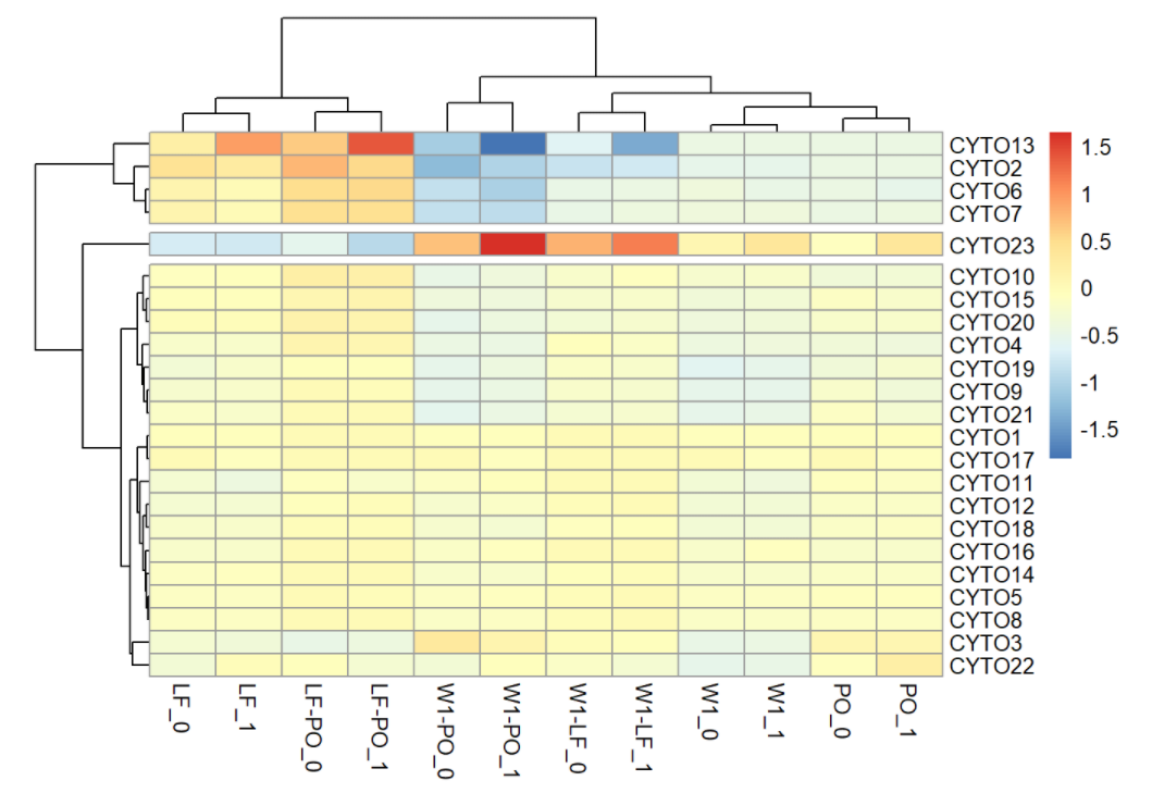
The rows of above heatmap shows 23 cytokines, the columns represent IRI status at different time point. The colors represent normalized median cytokine values (blue = low, red = high). The rows and columns are ordered based on the results of hierarchical clustering. Note that for illustration purpose, we set divided the rows into 3 clusters. As we can tell from the plot, the first cluster contained cytokine 13,2,6,7 and the second cluster contained only cytokine 23. Generally speaking, group with IRI has a higher normalized median cytokine levels in these two clusters. As for the cytokine 23, IRI+ group has larger difference of cytokine value between any two time points. The rest of cytokines are in the third cluster, which does not show a clear pattern.
Then we plot the histogram of INF and NEC values, grouped by IRI status
ggplot(df, aes(x=INF, color=IRI)) +
  geom_histogram(fill="white", position="dodge") + theme_bw()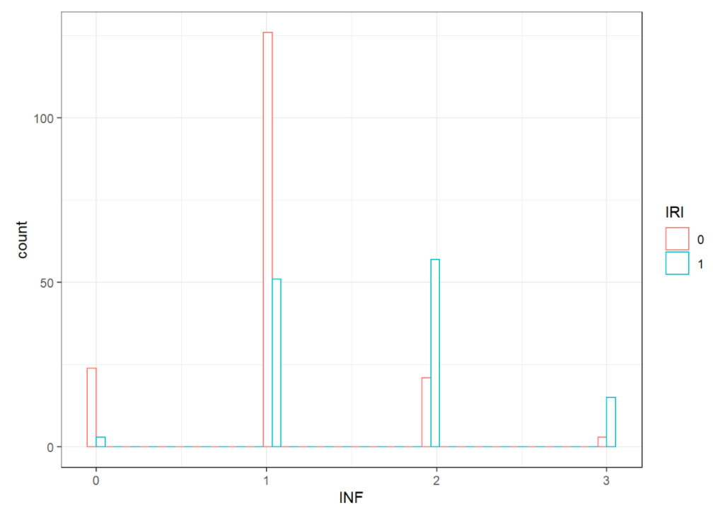
ggplot(df, aes(x=NEC, color=IRI)) +
  geom_histogram(fill="white", position="dodge") + theme_bw()
We can tell from the plots that most of IRI+ patients have a 2 INF level and 2 NEC level. Most of IRI- patients have a 1 INF level and 1 NEC level.
V. Variable assessment
V.I Log-transformation
df1 <- read.csv("402df.csv")

par(mfrow = c(3, 3))
hist(df1$CYTO1, main="CYTO1")
hist(df1$CYTO2, main="CYTO2")
hist(df1$CYTO3, main="CYTO3")
hist(df1$CYTO10, main="CYTO10")
hist(df1$CYTO11, main="CYTO11")
hist(df1$CYTO12, main="CYTO12")
hist(df1$CYTO18, main="CYTO18")
hist(df1$CYTO19, main="CYTO19")
hist(df1$CYTO20, main="CYTO20")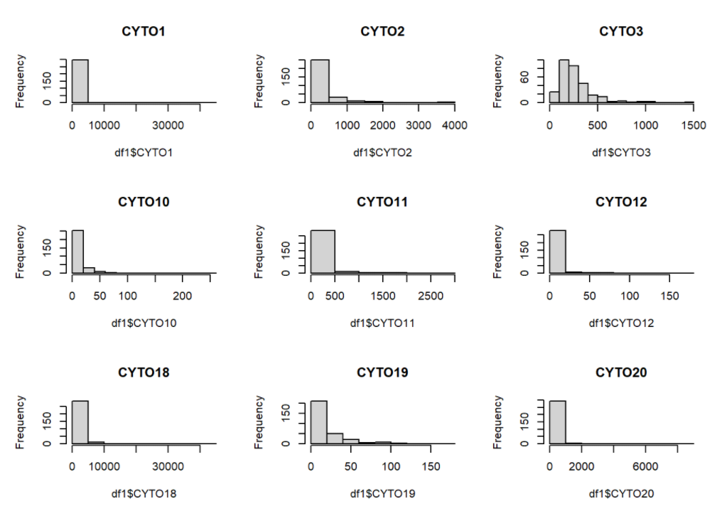
As we can see from the histograms of some of the histograms, there is a strong right skewness for all of the cytokine levels. Therefore, there exist a motivation to log-transform the data.
cols <- c("CYTO1","CYTO2", "CYTO3","CYTO4", "CYTO5","CYTO6", "CYTO7","CYTO8",
          "CYTO9","CYTO10", "CYTO11","CYTO12", "CYTO13","CYTO14", "CYTO15","CYTO16",
          "CYTO17","CYTO18", "CYTO19","CYTO20", "CYTO21","CYTO22", "CYTO23")
df1[cols] <- log(df1[cols])

par(mfrow = c(3, 3))
hist(df1$CYTO1, main="CYTO1")
hist(df1$CYTO2, main="CYTO2")
hist(df1$CYTO3, main="CYTO3")
hist(df1$CYTO10, main="CYTO10")
hist(df1$CYTO11, main="CYTO11")
hist(df1$CYTO12, main="CYTO12")
hist(df1$CYTO18, main="CYTO18")
hist(df1$CYTO19, main="CYTO19")
hist(df1$CYTO20, main="CYTO20")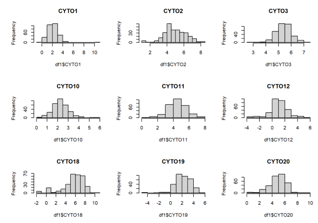
Now the selected histograms have improved significantly. We are going to proceed out analysis with the transformed dataset.
V.II Wilcoxon test
#Prepare data
df <- read.csv("402df.csv")
df_visual <- df %>% select(CYTO1:CYTO23)
df <- df %>% mutate(IRI=as.factor(IRI))
df[,paste0("CYTO",c(1:23))] <- log(df[,paste0("CYTO",c(1:23))])
df_dif <- df
df_dif[which(df_dif$Stype=="PO"), paste0("CYTO",c(1:23))] <-
  df_dif[which(df_dif$Stype=="LF"), paste0("CYTO",c(1:23))] -
  df_dif[which(df_dif$Stype=="PO"), paste0("CYTO",c(1:23))]
df_dif[which(df_dif$Stype=="LF"), paste0("CYTO",c(1:23))] <-
  df_dif[which(df_dif$Stype=="W1"), paste0("CYTO",c(1:23))] -
  df_dif[which(df_dif$Stype=="LF"), paste0("CYTO",c(1:23))]
df_dif[which(df_dif$Stype=="W1"), paste0("CYTO",c(1:23))] <-
  df_dif[which(df_dif$Stype=="W1"), paste0("CYTO",c(1:23))] -
  df_dif[which(df_dif$Stype=="PO"), paste0("CYTO",c(1:23))]
df_dif$Stype[which(df_dif$Stype=="W1")] <- "W1-PO"
df_dif$Stype[which(df_dif$Stype=="LF")] <- "W1-LF"
df_dif$Stype[which(df_dif$Stype=="PO")] <- "LF-PO"
Firstly, we evaluated each cytokine for its correlation with IRI outcome individually based on the Wilcoxon nonparametric rank-sum test.
# Wilcoxon nonparametric rank-sum test
df_test <- rbind(df, df_dif)
stat.test <- NULL
for(k in paste0("CYTO",c(1:23))){
  for(i in unique(df_test$Stype)){
  temp <- df_test %>%
    filter(Stype==i) %>%
    rename("CYTO" = k) %>%
    wilcox_test(CYTO ~ IRI) %>%
    add_significance() %>%
    mutate(Stype=i,var=k)
  stat.test <- rbind(stat.test, temp)
  }
}

stat.test[,-1] %>%
  select(var, Stype, group1:p.signif) %>%
  filter(p.signif!="ns") %>%
  kbl() %>%
  kable_classic(full_width = F, html_font = "Cambria")
As we can tell from the summary table, CYTO16 value in W1 stage and the change of CYTO16 value between W1 and LF stage are significant different between IRI+ and IRI- groups. In addition, CYTO22 value in LF stage are significant different between IRI+ and IRI- groups.
VI. Analysis of data set
VI.I Main effects
# Data preparation
df_1 <- df1 %>%
  group_by(PID) %>%
  filter(Stype == 'PO') %>%
  select(c(4, 8:30))

df_2 <- df1 %>%
  group_by(PID) %>%
  filter(Stype == 'LF') %>%
  select(c(4, 8:30))

df_3 <- df1 %>%
  group_by(PID) %>%
  filter(Stype == 'W1') %>%
  select(c(4, 8:30))

# Get their differences for each patient
df_1num <- df_1[, 4:25]
df_2num <- df_2[, 4:25]
df_3num <- df_3[, 4:25]
diff1 <- df_2num - df_1num
diff2 <- df_3num - df_2num
diff3 <- df_3num - df_1num

df_diff1 <- df_1
df_diff1[, 4:25] <- diff1

df_diff2 <- df_1
df_diff2[, 4:25] <- diff2

df_diff3 <- df_1
df_diff3[, 4:25] <- diff3
Then we can fit the model with main effects only:
# Before
mod1_before <- glm(IRI ~ .-PID, family = binomial, df_1)
  # No significant cytokine

# During
mod1_during <- glm(IRI ~ .-PID, family = binomial, df_2)
  # CTYO01, 02, 014 were significant

# After
mod1_after <- glm(IRI ~ .-PID, family = binomial, df_3)
  # CTYO22

# Difference 1
mod1_diff1 <- glm(IRI ~ .-PID, family = binomial, df_diff1)
  # CTYO04, 09, 014 were significant

# Difference 2
mod1_diff2 <- glm(IRI ~ .-PID, family = binomial, df_diff2)
    # CTYO09

# Difference 3
mod1_diff3 <- glm(IRI ~ .-PID, family = binomial, df_diff3)
  # No significant cytokine
After fitting the logistic models with only the main effect, CTYO01, 02, 09, 014, 022 have shown significance.
VI.II With interactions
Then we include all the two-way interactions between cytokines to test whether cytokines influence IRI together. In order to arrive at a more parsimonious model, we simplified the model by a elastic net selection algorithm. Elastic net linear regression applied the penalties that from both the lasso and ridge techniques to regularize regression models. It combines both the lasso and ridge regression methods and improve the shortcomings of these two methods. The technique is appropriate where the dimensional data is greater than the number of samples used. Note that we build the model based on each Stype (PO, LF, W1, LF-PO, W1-LF, W1-PO) independently.
# log the data
df_test2 <- model.matrix(~.^2-1,df_test[,paste0("CYTO",c(1:23))])
glm_results <- NULL
for(i in unique(df_test$Stype)){
  # logit regression
  set.seed(1996)

  y <- df_test %>% filter(Stype==i) %>% select(IRI) %>% as.matrix
  x <- df_test2[which(df_test$Stype==i),] %>% as.matrix

  cv.lasso <- cv.glmnet(x, y, family = "binomial")
  #plot(cv.lasso)
  model <- glmnet(x, y, family = "binomial",
                  lambda = cv.lasso$lambda.1se)
  ind <- abs(coef(model)[,ncol(coef(model))])>0.000000000
  vars.selected <- rownames(coef(model))[ind]
  vars.selected <- vars.selected[-which(vars.selected == "(Intercept)")]

  df_final <- data.frame(as.numeric(y), x[,vars.selected])
  names(df_final) <- c("y", vars.selected)
  glm(y~., data=df_final,
      family=binomial) %>% summary %>%
    .$coefficients %>% as.data.frame -> temp
  temp$var <- row.names(temp)
  glm_results <- rbind(glm_results, data.frame(Stype=i, temp))
}
colnames(glm_results)[c(3,5)] <- c("sd","p-value")
glm_results <- glm_results[which(grepl("(Intercept)",
                                       row.names(glm_results))==F),]
glm_results[,2:5] <- glm_results[,2:5] %>% round(3)
row.names(glm_results)<-NULL
Following is the summary table for models,
glm_results %>%
  select("var","Stype","Estimate","sd","z.value","p-value") %>%
  kbl() %>%
  kable_classic(full_width = F, html_font = "Cambria")
As we can tell from the model summary, CYTO23 is proved to be significant different between IRI+ and IRI- groups at PO stage (p = .035). CYTO22 appears to be different between IRI+ and IRI- groups at LF stage (p = .065). We also found that there exists significant interaction effect between the CYTO5 (change between LF and PO stage) and CYTO8 (change between LF and PO stage) between IRI+ and IRI- groups (p = .022). Interaction effect between the CYTO12 (change between W1 and LF stage) and CYTO14 (change between W1 and LF stage) between IRI+ and IRI- groups (p = .038) is also significant.
VI.III NEC/INF
For the next section, we analyzied the correlation between re-transplant cytokines and after-transplant by spearman correlation
#data processing
df <- read.csv("402df.csv")
df[,"INF"] <- as.factor(df[,"INF"])
df[,"NEC"] <- as.factor(df[,"NEC"])
pre_index <- seq(1,300,3)
after_index <- seq(3,300,3)
df_test <- NULL
df_test$INF_after <- df[after_index,"INF"]
df_test$NEC_after <- df[after_index,"NEC"]
df_test <- cbind(df_test, df[pre_index,paste0("CYTO",c(1:23))])
df_test[,paste0("CYTO",c(1:23))] <- log(df_test[,paste0("CYTO",c(1:23))])
We apply the spearman correlation (Koelman) with INF and NEC as factors, we see no strong correlations between INF and NEC after transplant with Cytokines before transplant nor are they significant.
correlation::correlation(df_test[1:2], df_test[3:25], method = "spearman",
                         include_factors = TRUE)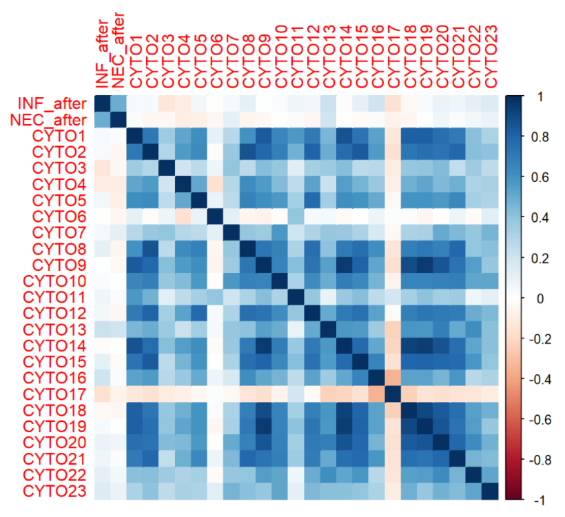
Visualize the correlation to see the weak correlations between cytokines and INF/NEC score.
Note here NEC and INC are treated as numeric variables.
df_test[,"INF_after"] <- as.numeric(df_test[,"INF_after"])
df_test[,"NEC_after"] <- as.numeric(df_test[,"NEC_after"])
corrplot(cor(df_test,method = "spearman"),
  method = "color")
VII. Interpretation of results
According to all the results above, we can conclude that,
- Cytokine 23 has significant influence on IRI individually at
POstage. - Cytokine 01, 02, 14, 22 have significant influence on IRI individually at
LFstage. - Cytokine 16, 22 have significant influence on IRI individually at
W1stage. - Cytokine 4, 9, 14 have significant influence on IRI individually at
LF-POstage (change betweenLFandPOstage). - Cytokine 9, 16 have significant influence on IRI individually at
W1-LFstage (change betweenW1andLFstage). - Interaction effect between the Cytokine 5 and 8 has significant influence on IRI individually at
LF-POstage (change betweenLFandPOstage). - Interaction effect between the Cytokine 12 and 14 has significant influence on IRI individually at
W1-LFstage (change betweenW1andLFstage). - There is no significant correlation between pre-transplant cytokines and after-transplant NEC/INF.
VIII. Limitation
Lack of the demographic data and clinical parameters, results may be affected by confounders.
The results can be affected at individual level. If we could get more recordings from each patients, maybe we could fit random effects model to adjust for that.
Further research (pathological) are needed to provide a solid conclusion about casual relationship between Cytokine and IRI status.