Goals of analysis

The study objective is to examine the association of individual’s systolic blood pressure (SBP) with family history of hypertension, the day of test (working days or not) and menstrual cycle phase. We are also interested in whether interaction between day of test and family history affect the SBP.

Data

The data set contains 203 female nurse’s systolic blood pressure (SBP) (in mmHG) test results. Each person has multiple SBP readings. There are three predictors to included in the data set: famhist, work and phase. Note that variable famhist has three levels in the original data set (0 = no parents, 1 = one parent, 2 = two parents with hypertension). Since research suggested that affects of the family history of hypertension is not linear, we convert famhist to two dummy variable fam1 (one parents with hypertension or not) and fam2 (two parents with hypertension or not), taking the group with no hypertensive family member as the reference. Then we formed a interactive term of famhist and work. Please note that we re-coded the famhist situation as a binary variable when generating the interactive term for the convenience (0: no parents with hypertension, 1: have hypertensive family members).

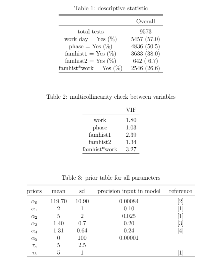
Since all of the variables are binary, there was no outlier within the predictors. Table 1 presents the descriptive statistics of the whole dataset. In order to prevent the model estimation from being distorted due to the high correlation between variables, we calculated the coefficient of variance expansion (VIF) of each factor. Table 2 presents that there is little multiple multicollinearity between variables. Thus, we are safe to put data into the model.

The model

We will use linear regression with random effects to model this data. We denoted \(k^{\text{th}}\) systolic blood pressure (SBP) test result for the \(i^{\text{th}}\) nurse by \(y_{ik}\). The proposed model is: \[\begin{equation} \mu_{ik} = \beta_i+\alpha_0+\alpha_1 \text{Fam1}_{ik}+\alpha_2 \text{Fam2}_{ik}+\alpha_3 \text{Work}_{ik}+\alpha_4 \text{Phase}_{ik}+\alpha_5 \text{Fam*work}_{ik} \end{equation}\] where \(i\) runs from 1 to 203, \(k\) runs from 1 to 9573. The random effect terms \(\beta_i|\tau_b\sim N(0,\tau_b)\) are independent and identically distributed given precision \(\tau_b\). Interception parameter \(\alpha_0\) is assumed normal distributed. Note that \(\alpha_0\) represents baseline SBP level that is not recorded on week day nor within the phase for individuals who has no parents with hypertension. Parameters \(\alpha_1\sim\alpha_5\) are regression coefficients and also are assumed normal distributed. We assumed that SBP values follows a normal distribution with mean \(\mu_{ik}\) and precision \(\tau_e\) (Eqn 2).

\[\begin{equation} y_{ik}\sim N(\mu_{ik},\tau_e) \end{equation}\]

Prior information

The priors for most of parameters are decided based on past reseach. Marczak et al. suggested that average systolic blood pressure in a group consisted of 125 healthy persons has mean 119.7 and standard deviation 10.9 mmHg. Here we approximate this value as the baseline level in or model. Tozawa et al. collected 9,914 individuals information and suggested that persons that have one and two hypertensive family members have an average of 2 and 5 mmHg higher SBP than that of persons that have none hypertensive family members, respectively. In addition, research shows adjusted systolic blood pressure was higher in the follicular than in the luteal phase (mean difference 1.31 mmHg, sd 0.64 mmHg). Systolic BP was lower during the weekend than on Monday (mean difference 1.4 mmHg). We used independent priors to do the analysis and assumed \(\alpha_0\sim \alpha_5\) to be normal distributed and \(\tau_e,\tau_b\) be Gamma distributed. Please note that some researches do not provide sds and we just applied the Range Method to estimate a sd. In addition, we assigned a vague range for \(\alpha_5\), the coefficient of interactive term. Then, based on the influence we would like the prior data to have, we weight the prior precision to be \(\frac{1}{10}\), rather than using their original value directly (Table 3).

Results and conclution

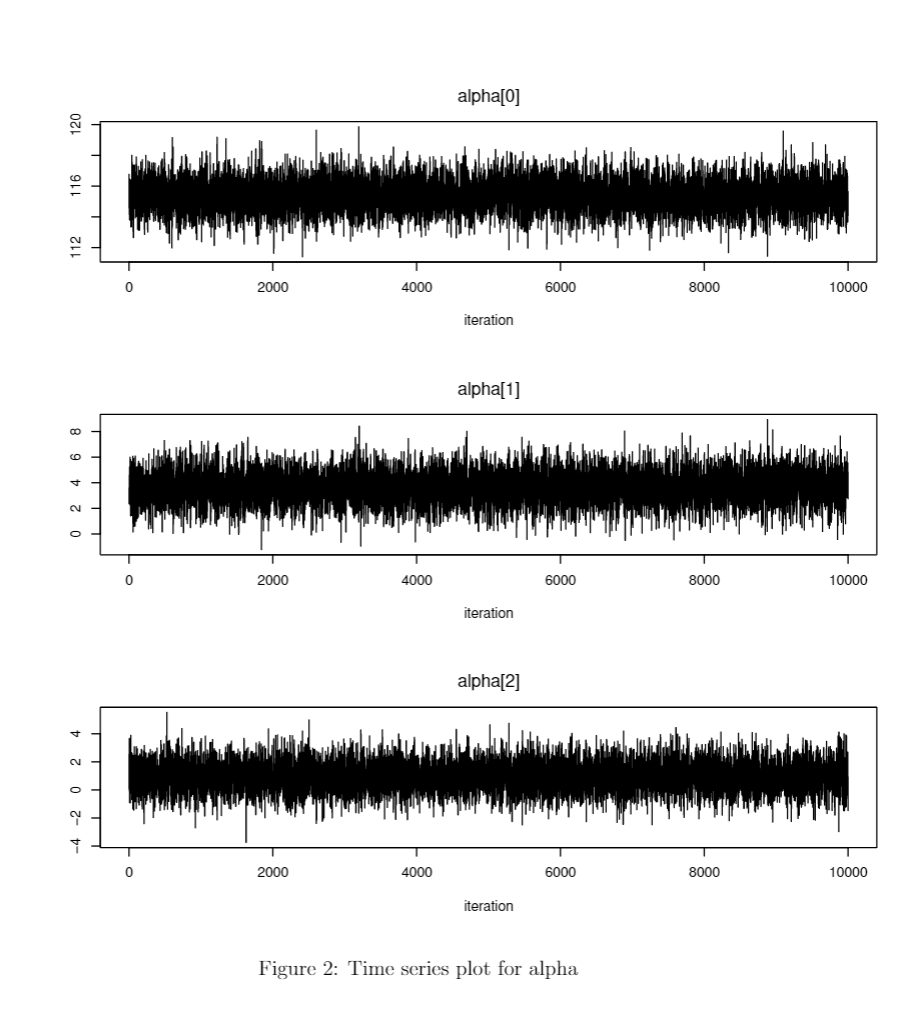
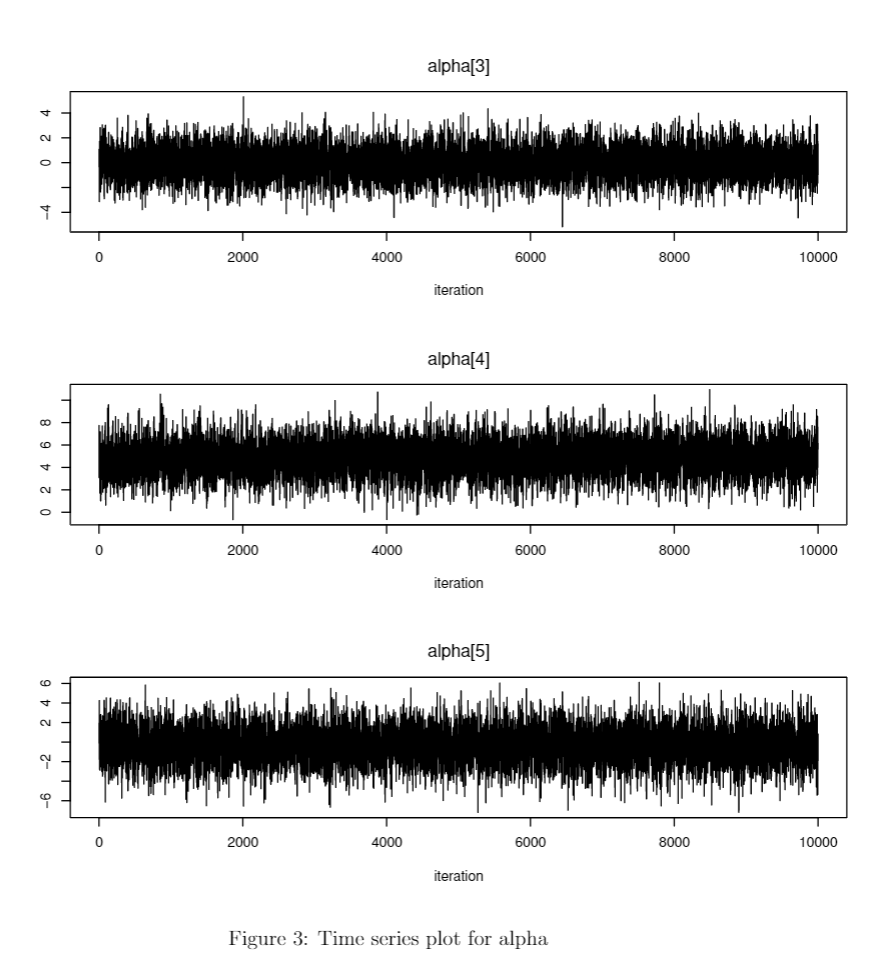
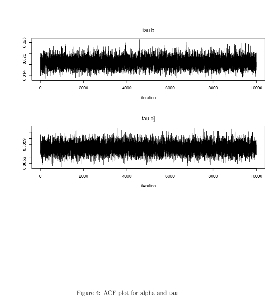
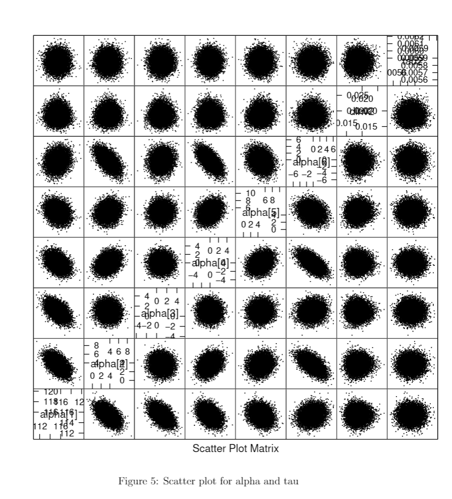
For the regression coefficients (Figure 1), all of alphas’ the auto-correlations hit zero within around 10 lags. And the time series plot (Figure 2 & 3) also show that all of alpha converge well. In addition, Figure 1 & 4 illustrate that \(\tau_e\) and \(\tau_b\) converge well. According to the scatter plot (Figure 5), we found that there are little correlations within regression coefficients.

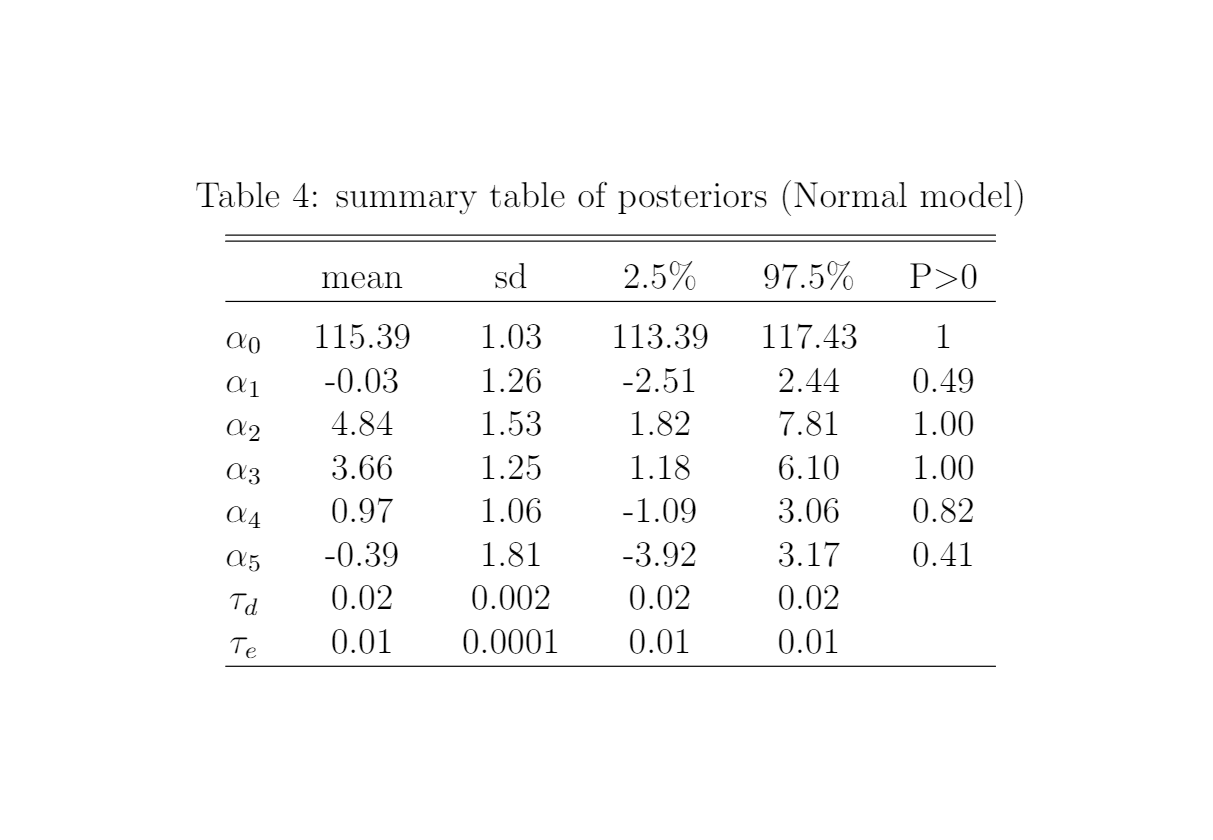
Table 4 presents the key results of estimated posteriors. We can tell from the table that estimated average baseline SBP level that is not recorded on week day nor within the phase for individuals who has no parents with hypertension is 115.39 (sd: 1.03). Patients has two parents with hypertension are estimated to have 4.84 mmHG higher SBP (under 99% probability), while SBP of patients has one parent with hypertension shows no significant difference, compared to patients has none parent with hypertension. Individuals are proved to have a average 3.66 mmHG higher SBP on working days (under 99% probability). Menstrual cycle phase does not have significant effects on the SBP, and interaction of the work and family hypertension history does not significantly affect the SBP level as well.

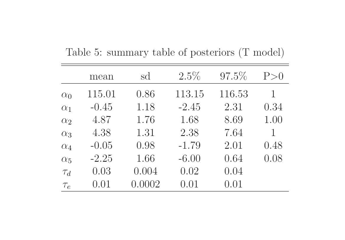
For the sensitivity analysis, we applied a T-model with the 4 degrees of freedom on the data, rather than the normal model. Table 5 presents the summary of estimated posteriors, we found that it provides largely consistent results as the normal model, which shows that our analysis is robust.

Appendix