Data science practice 4

Q1.0

Read following tutorials on the R package miceRanger for imputation: https://github.com/farrellday/miceRanger, https://cran.r-project.org/web/packages/miceRanger/vignettes/miceAlgorithm.html.

A more thorough book treatment of the practical imputation strategies is the book [*_Flexible Imputation of Missing Data_*](https://stefvanbuuren.name/fimd/) by Stef van Buuren. 

Q1.1

Explain the jargon MCAR, MAR, and MNAR.

solution:

• MAR: missing at random. The absence of data was independent of incomplete variables as well as complete variables.
• MCAR: missing completely at random. The absence of data relies solely on the complete variable.
• MNAR: missing not at random. The absence of data in the incomplete variables relies on the incomplete variables themselves and such absence is not negligible.

Q1.2

Explain in a couple of sentences how the Multiple Imputation by Chained Equations (MICE) work.

solution: operates under the assumption that given the variables used in the imputation procedure, the missing data are Missing At Random (MAR). In the MICE procedure a series of regression models are run whereby each variable with missing data is modeled conditional upon the other variables in the data. This means that each variable can be modeled according to its distribution. reference link

Q1.3

Perform a data quality check of the ICU stays data. Discard variables with substantial missingness, say >5000 NAs. Replace apparent data entry errors by NAs.

Please note that here we dropped variables that have more than 7000 NAs. In addition, we assigned the outliers (out of 1.5*IQR range) of each numeric variables as NA.

#define functions
.quantile_cut <- function(x){
  lb <- quantile(df[, x] , 0.25, na.rm = TRUE)
  ub <- quantile(df[, x] , 0.75, na.rm = TRUE)
  iqr <- ub - lb
  df[which(df[, x] <= lb - 1.5*iqr | df[, x] >= ub + 1.5*iqr), x] <- NA
  return(df[,x])
}
.na_count <- function(x, data = icu_cohort){
  na_num <- which(is.na(data[, x]) == T) %>% length()
}


icu_cohort <- readRDS("./icu_cohort.rds")
var_list <- c("first_careunit",  
"los", "gender", "admission_type", "admission_location", 
"insurance", "language", "marital_status", 
"ethnicity", "age_at_adm", "bicarbonate", "calcium", "chloride", 
"creatinine", "glucose", "magnesium", "potassium", "sodium", 
"hematocrit", "wbc", "lactate", "heart_rate", 
"non_invasive_blood_pressure_systolic", "non_invasive_blood_pressure_mean",
"respiratory_rate", "temperature_fahrenheit", 
"arterial_blood_pressure_systolic", 
"arterial_blood_pressure_mean")


var_list <- var_list[which(apply(var_list %>% 
                                   as.matrix, 1, .na_count) <= 7000)]

icu_cohort %>% 
  select(all_of(var_list)) -> df
name_list <- names(df %>% select_if(is.numeric))[-c(1, 2)] %>% as.list()
numeric_var <- lapply(name_list, .quantile_cut) %>% Reduce("cbind", .)
df <- df %>% 
  select(!is.numeric) %>%
  cbind(numeric_var)

Q1.4

Impute missing values by miceRanger (request \(m=3\) datasets). This step is very computational intensive. Make sure to save the imputation results as a file.

Note that we didn’t include the age_at_adm in the multiple imputation, beacase 1) it has no missing value in original data set; 2) it does not converge in the miceRanger; 3) it may also influence the converge of other variabls. We also removed death_30 and discharge location and hospital expire flag since they contain the information of response (survival/dead), part of which is supposed to be unknown in the predicting part.

# Set up back ends.
cl <- makeCluster(detectCores())
registerDoParallel(cl)

miss_list <- names(df)[which(apply(names(df) %>% as.matrix,
                                   1, .na_count, data = df) > 0)]

# Perform mice 
parTime <- system.time(
  miceObjPar <- miceRanger(
      df
    , m = 3
    , maxiter = 7
    , vars = miss_list
    , max.depth = 15
    , parallel = TRUE
    , verbose = TRUE
  )
)
stopCluster(cl)
registerDoSEQ()

saveRDS(miceObjPar, file = "./miceObjPar.rds")

Q1.5

Make imputation diagnostic plots and explain what they mean.

miceObjPar <- readRDS("./miceObjPar.rds")
plotDistributions(miceObjPar, vars = 'allNumeric')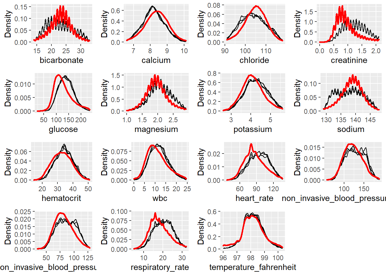

This is the Distribution of Imputed Values plots, the red line is the density of the original, nonmissing data. The smaller, black lines are the density of the imputed values in each of the datasets. According to the plots, we found that the imputed distributions is largely consistent to the original distribution for each variable. It means that the data was Missing Completely at Random (MCAR).

plotCorrelations(miceObjPar, vars = 'allNumeric')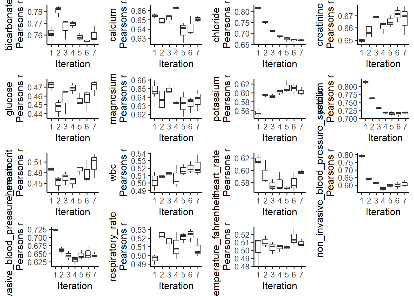

The Convergence of Correlation plots shows boxplots of the correlations between imputed values in every combination of datasets, at each iteration. We can see that imputation for all of variables converged after 5 interactions.

plotVarConvergence(miceObjPar, vars='allNumeric')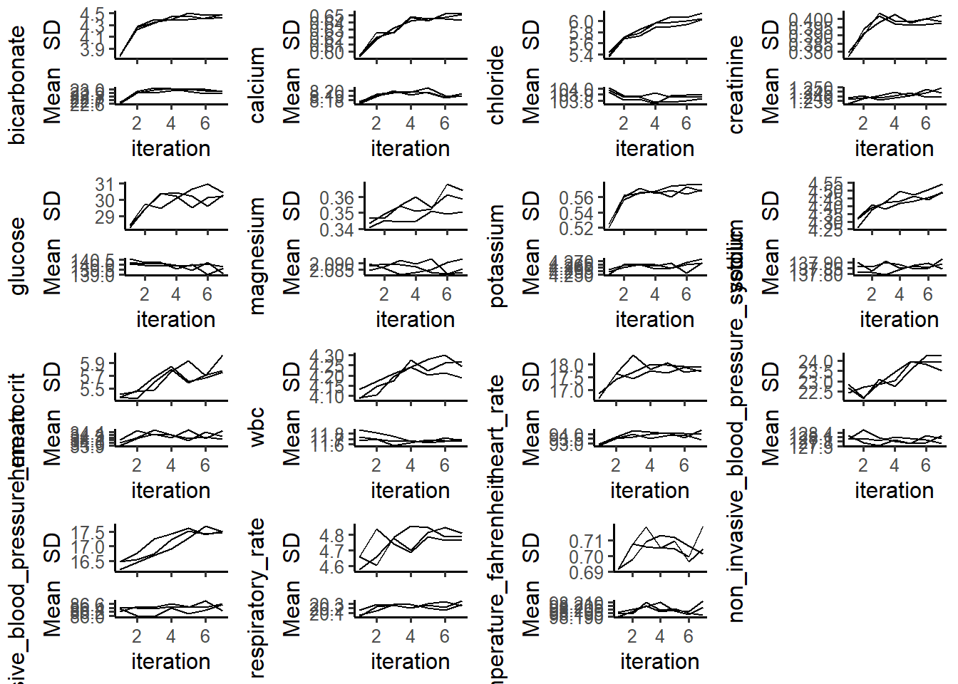

The Center and Dispersion Convergence plots were designed to see whether the missing data locations are correlated with higher or lower values. From the plots, we can see that the most of imputed data were largely converged to the true theoretical mean, while non_invasive_blood_pressure seems have a slight convergence issue. We would ignore it at current stage.

plotModelError(miceObjPar, vars = 'allNumeric')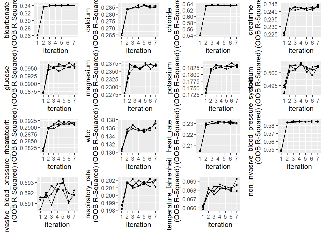

According to the plots of OOB accuracy for Random Forests model classification. We can see how these converged as the iterations progress: It looks like the variables were imputed with a reasonable degree of accuracy after 5 iterations.

Q1.6

Obtain a complete data set by averaging the 3 imputed data sets.

.dummy_trans <- function(x){
  out <- dummy_cols(x,
           remove_first_dummy = TRUE,
           remove_selected_columns = TRUE)
  return(out)
}

dataList <- completeData(miceObjPar)
Datasets_imputed <- lapply(dataList, .dummy_trans)

Final_data <- (Datasets_imputed[["Dataset_1"]] +
  Datasets_imputed[["Dataset_2"]] +
  Datasets_imputed[["Dataset_3"]])/3 

df <- Final_data %>%
  mutate_at(vars('first_careunit_Coronary Care Unit (CCU)' : 
                   'ethnicity_WHITE'), round) 

Q2.1 Data preparation

Partition data into 80% training set and 20% test set. Stratify partitioning according the 30-day mortality status.

df <- df %>%
  select(contains(c("gender", "ethnicity", "marital")) |
           bicarbonate : temperature_fahrenheit) %>%
  mutate(age = icu_cohort$age_at_adm)

names(df)[c(3, 4, 6)] <- c("ethnicity_BLACK", "ethnicity_HISPANIC",
                          "ethnicity_UNABLE")

set.seed(19969)
folds <- createFolds(factor(icu_cohort$death_30), k = 5, list = T)

#test data set
data.test.x <- df[folds[[1]], ] %>% 
  mutate_at(vars(bicarbonate : age), scale) %>% as.matrix()
data.test.y <- dummy_cols(icu_cohort$death_30[folds[[1]]],
           remove_first_dummy = TRUE,
           remove_selected_columns = TRUE) %>% as.matrix()
#train data set
data.train.x <- df[folds[-1] %>% Reduce("c", .), ] %>% 
  mutate_at(vars(bicarbonate : age), scale) %>% as.matrix()
data.train.y <- dummy_cols(icu_cohort$death_30[folds[-1] %>% Reduce("c", .)],
           remove_first_dummy = TRUE,
           remove_selected_columns = TRUE) %>% as.matrix()

Q2.2 Modeling

Train the models using the training set.

We noticed that the data set is heavily imbalanced, which may cause the problem of low prediction accuracy for death_30 cases. Considering that a major goal of the prediction model may be sending early warning to cases which has a higher risk of death, we tryed to increase the prediction accuracy for death_30 cases by using the weighting and resampling method in two models.

• Method 1

neural network (MLP) [original weight]

model <- keras_model_sequential() 
model %>% 
  layer_dense(units = 16, activation = 'relu',
              kernel_initializer = "uniform", input_shape = c(27)) %>% 
  layer_dropout(rate = 0.4) %>% 
  layer_dense(units = 8, activation = 'relu',
              kernel_initializer = "uniform") %>%
  layer_dropout(rate = 0.3) %>%
  layer_dense(units = 1, activation  = "sigmoid")
summary(model)
model %>% compile(
  loss = 'binary_crossentropy',
  optimizer = 'adam',
  metrics = c('accuracy')
)
set.seed(19969)
system.time({
history1 <- model %>% fit(
  data.train.x, data.train.y, 
  epochs = 30, batch_size = 128, 
  validation_split = 0.3
)
})

model %>% evaluate(data.test.x, data.test.y)
results1 <- model %>% predict_proba(data.test.x) 
saveRDS(results1, "./results1.rds")
saveRDS(history1, "./history1.rds")

Check the confusionMatrix and history plots of prediction results

results1 <- readRDS("./results1.rds")
history1 <- readRDS("./history1.rds")
confusionMatrix (results1 %>% round %>% as.factor, 
                 as.matrix(data.test.y) %>% as.factor)
plot(history1)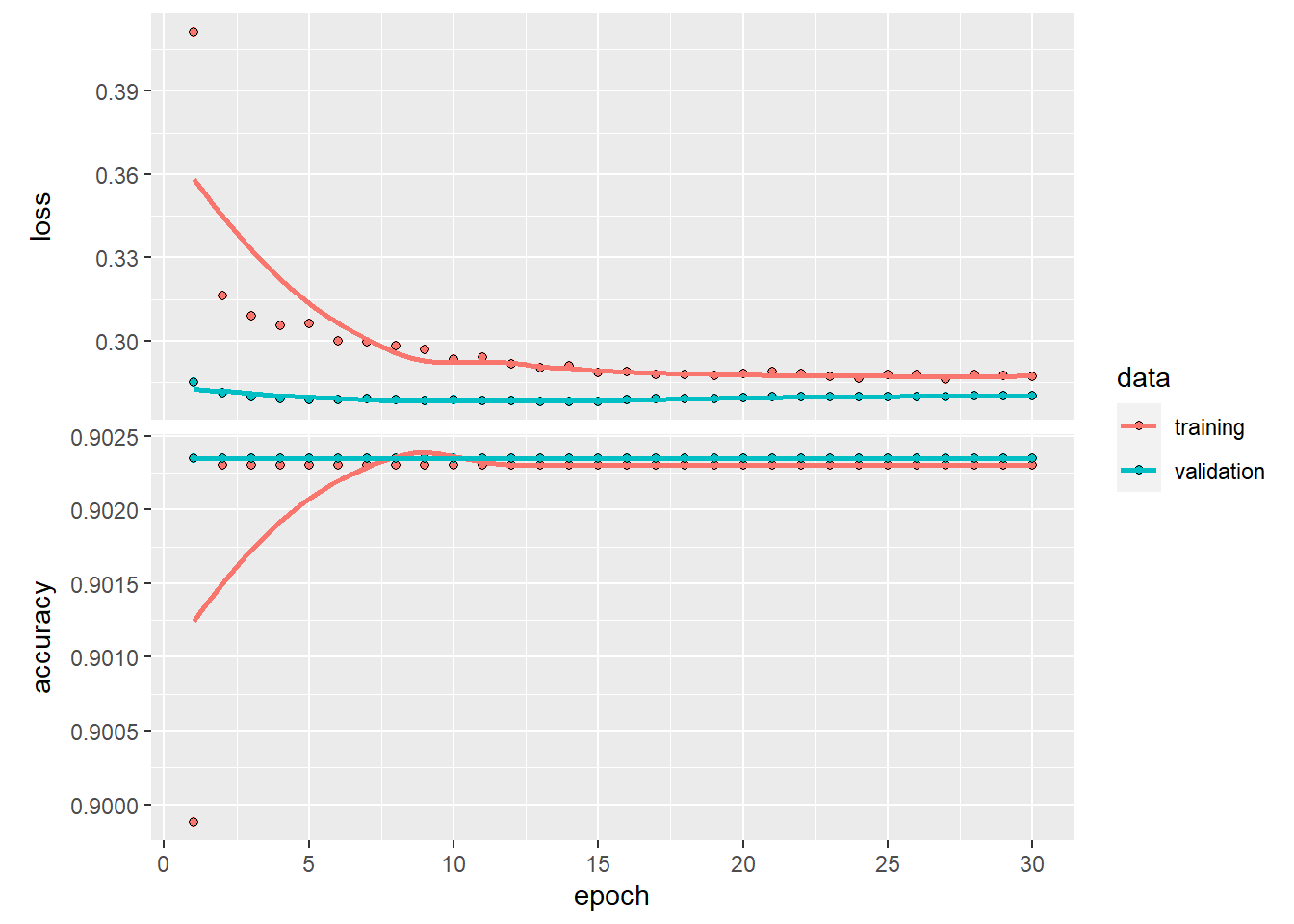

We can see from the history plot that the original model (without weighting and bias_initializer) converge very quick. It provided a high accuracy for the non death_30 cases, while the predicted accuracy for death_30 cases is terribly low.

Then we tried to add weighting in the model. We also set a initializing weight for the MLP model to help model converge.

• Method 1.1

neural network (MLP) [with weighting and bias_initializer]

model <- keras_model_sequential() 
model %>% 
  layer_dense(units = 64, activation = 'relu',
              bias_initializer = initializer_constant(0.01),
              kernel_initializer = "uniform", input_shape = c(27)) %>% 
  layer_dropout(rate = 0.4) %>% 
  layer_dense(units = 32, activation = 'relu',
              bias_initializer = initializer_constant(0.01),
              kernel_initializer = "uniform") %>%
  layer_dropout(rate = 0.3) %>%
  layer_dense(units = 1, activation  = "sigmoid")
summary(model)
model %>% compile(
  loss = 'binary_crossentropy',
  optimizer = 'adam',
  metrics = c('accuracy')
)
set.seed(199609)
system.time({
history2 <- model %>% fit(
  data.train.x, data.train.y, 
  epochs = 700, batch_size = 128, 
  class_weight = list("0" = 1, "1" = 8), 
  validation_split = 0.3
)
})

model %>% evaluate(data.test.x, data.test.y)
results2 <- model %>% predict_proba(data.test.x) 
saveRDS(results2, "./results2.rds")
saveRDS(history2, "./history2.rds")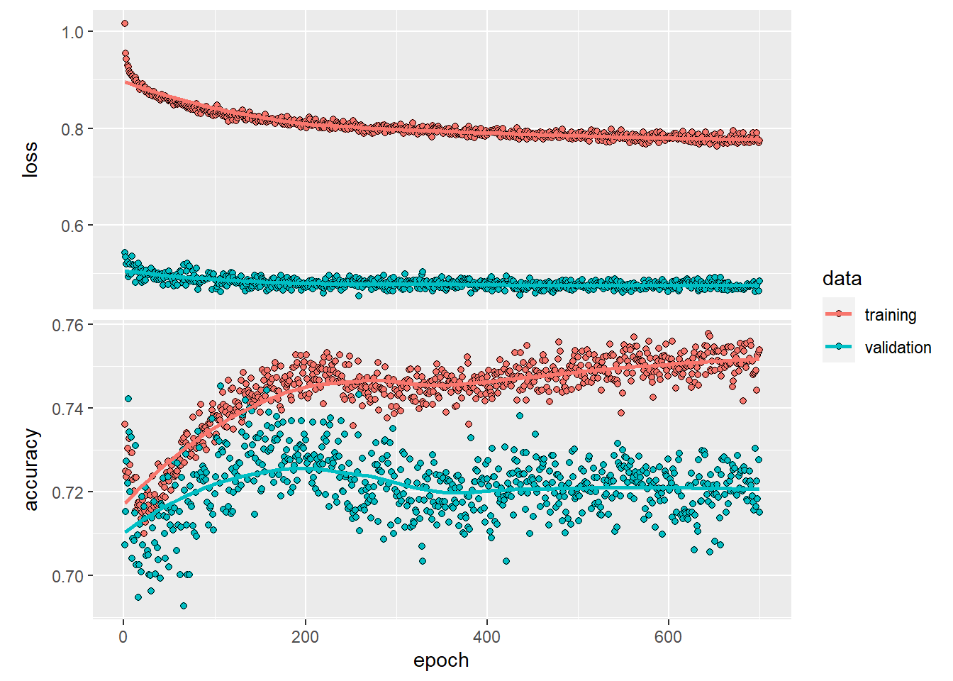

Check the confusionMatrix and history plots of prediction results

results2 <- readRDS("./results2.rds")
history2 <- readRDS("./history2.rds")
confusionMatrix (results2 %>% round %>% as.factor, 
                 as.matrix(data.test.y) %>% as.factor)
plot(history2)

We can tell from the history plots that the model converged after around 400 epochs (the validation line became stable).

• Method 2

XGBoost model [with variable selection and re-sampling]

In this model, we created relatively balanced samples (survival:dead = 3:1) by random under-sampling method.

###### model function ########
.importance_function <- function(dtrain){
  model <- xgboost(data = dtrain,          
                   nround = 500,
                   early_stopping_rounds = 30,
                   objective = "binary:logistic",
                   eval_metric = "logloss",
                   verbose = 0)
  importance_matrix <- xgb.importance(model = model) 
  return(importance_matrix)
}

.auc_function_train <- function(folds){
  dtrain <- xgb.DMatrix(data = b.train.x[-folds, ] %>% as.matrix(),
                        label= b.train.y[-folds] %>% as.matrix())
  dtest <- xgb.DMatrix(data = b.train.x[folds, ] %>% as.matrix(),
                       label= b.train.y[folds] %>% as.matrix())
  test_labels <- b.train.y[folds]
  
  model <- xgboost(data = dtrain,          
                   nround = 500,
                   early_stopping_rounds = 30, 
                   objective = "binary:logistic",
                   eval_metric = "logloss",
                   verbose = 0)
  pred <- predict(model, dtest) 
  xgbpred <- ifelse (pred >= 0.5,1,0)
  roc_l <- roc(test_labels,pred)
  auc_value <- auc(roc_l)
  return(auc_value)
}

.model_function_Total <- function(importance=F,auc=T){
  if(importance==T){
    cv.group.x <- lapply(folds,function(x){out<-NULL;
    out<-rbind(out,data.frame(label = b.train.y[-x], b.train.x[-x,]))})
    cv.group.y <- lapply(folds,function(x){out<-NULL;
    out<-rbind(out,data.frame(label = b.train.y[x], b.train.x[x,]))})
    
    dtrain <- lapply(cv.group.x, 
                     function(x){out <- xgb.DMatrix(data = x %>% as.matrix() 
                                                    %>% .[,-1],
                                                    label= x %>% as.matrix()
                                                    %>% .[,1])})
    dtest <- lapply(cv.group.y, 
                    function(x){out<-xgb.DMatrix(data = x %>% as.matrix()
                                                 %>% .[,-1],
                                                 label= x %>% as.matrix() 
                                                 %>% .[,1])})
    importance_matrix <- lapply(dtrain, .importance_function) 
    importance_combine <- Reduce("rbind", importance_matrix)
    return(importance_combine)
  }else if(auc==T){
    auc_value <- sapply(folds, .auc_function_train) #%>% mean() 
    auc_value_combine <- c(auc_value_combine, auc_value)
    return(auc_value_combine)
  }
}

Firstly we tried to rank the importance of all variables by 10-folder cross validation

importance_combine <- NULL
temp <- cbind(data.train.y,data.train.x) %>% as.data.frame()

for(i in 1:300){
  set.seed(1e7-i)
  data.balanced <- ovun.sample(.data_Yes~., data = temp, p = 0.33,
                               method = "under")$data
  b.train.x <- data.balanced[, -1] %>% as.matrix()
  b.train.y <- data.balanced[, 1] %>% as.matrix()
  folds <- createFolds(factor(b.train.y), k = 10, list = T)
  importance_combine <- rbind(importance_combine,
                              .model_function_Total(importance = T, auc = F))
  print(i)
}

importance_combine %>%
  group_by(Feature) %>%
  summarise(mean = mean(Gain)) %>%
  arrange(desc(mean)) -> importance_sum

saveRDS(importance_sum, "importance_sum.rds")

Check the plot of top 10 important variables

importance_sum <- readRDS("importance_sum.rds")
ggplot(data = importance_sum[1:10, ],
       mapping = aes(x = reorder(Feature, -mean), y = mean, fill=Feature))+
  geom_bar(stat = "identity")+
  scale_fill_brewer(palette = "RdBu") +
  xlab(NULL)+
  ylab("Relative Rmpotortance")+
  theme_few()+
  theme(axis.ticks.x = element_blank(),
        axis.text.x = element_blank())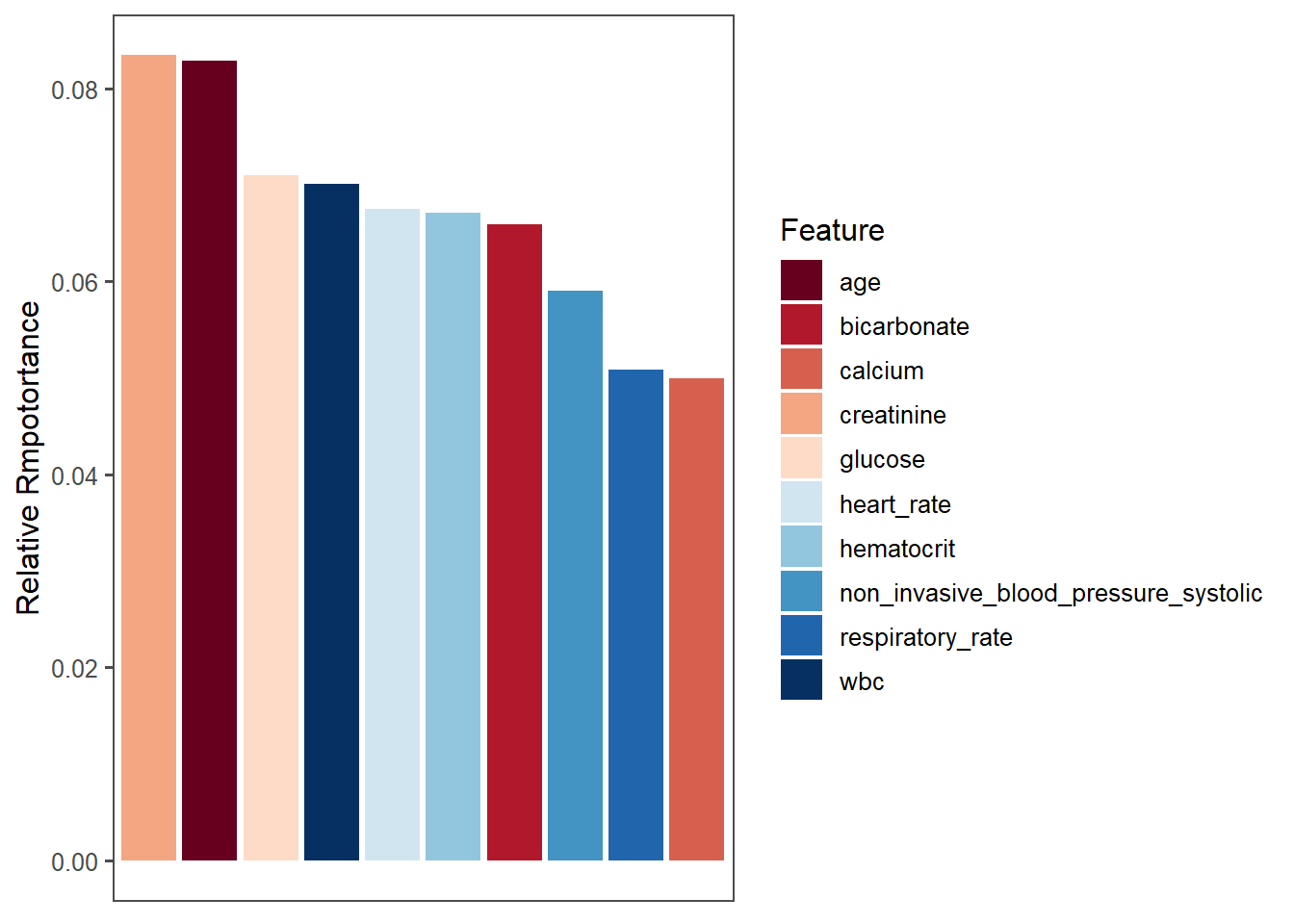

Then we did a forward-stepwise variable selection according to the AIC value (10-folder cross validation average).

feature_select<-NULL;auc.comb<-NULL
for(f in 1:15) {
  auc_value_combine<-NULL
  feature_select<-importance_sum$Feature[1:f]
  temp <- cbind(data.train.y, 
                data.train.x[,feature_select]) %>% as.data.frame()
  
  for(i in 1:100){
    set.seed(1e7-i)
    data.balanced <- ovun.sample(.data_Yes~., data = temp, p = 0.33,
                                 method = "under")$data
    b.train.x <- data.balanced[,-1] %>% as.matrix()
    b.train.y <- data.balanced[,1] %>% as.matrix()
    folds <- createFolds(factor(b.train.y), k = 10, list = T)
    auc_value_combine <- .model_function_Total(importance=F,auc=T)
    #print(paste0(f," variables - ", i, "%"))
  }
  
  auc_new <- auc_value_combine %>% mean()
  auc_sd <- auc_value_combine %>% sd()
  auc.comb <- rbind(auc.comb, data.frame(auc_new, auc_sd,model=f))
}
feature_select <- feature_select[1 : which.max(auc.comb$auc_new)] %>% 
  as.character()
saveRDS(feature_select, "./feature_select.rds")

Check the variables in the final model

feature_select <- readRDS("./feature_select.rds")
print(feature_select)

Finally, we trained the dataset (re-sampled) and predicted.

temp <- cbind(data.train.y, 
                data.train.x[, feature_select]) %>% as.data.frame()
data.balanced <- ovun.sample(.data_Yes~., data = temp, p = 0.33, 
                                seed = 199609, method = "under")$data
dtrain <- xgb.DMatrix(data = data.balanced[,-1] %>% as.matrix(),
                      label= data.balanced[,1] %>% as.matrix())
dtest <- xgb.DMatrix(data = data.test.x[, feature_select] %>% as.matrix(),
                      label= data.test.y %>% as.matrix())
model <- xgboost(data = dtrain,
                 nround = 500,
                 early_stopping_rounds = 30,
                 objective = "binary:logistic", 
                 eval_metric = "logloss",
                 verbose = 0)
xgbpred <- predict(model, dtest)
saveRDS(xgbpred, "./xgbpred.rds")

check the prediction results

xgbpred <- readRDS("./xgbpred.rds")
confusionMatrix(xgbpred %>% round %>% as.factor(), 
                 data.test.y %>% as.factor())

Q2.3 Comparation

Compare model prediction performance on the test set.

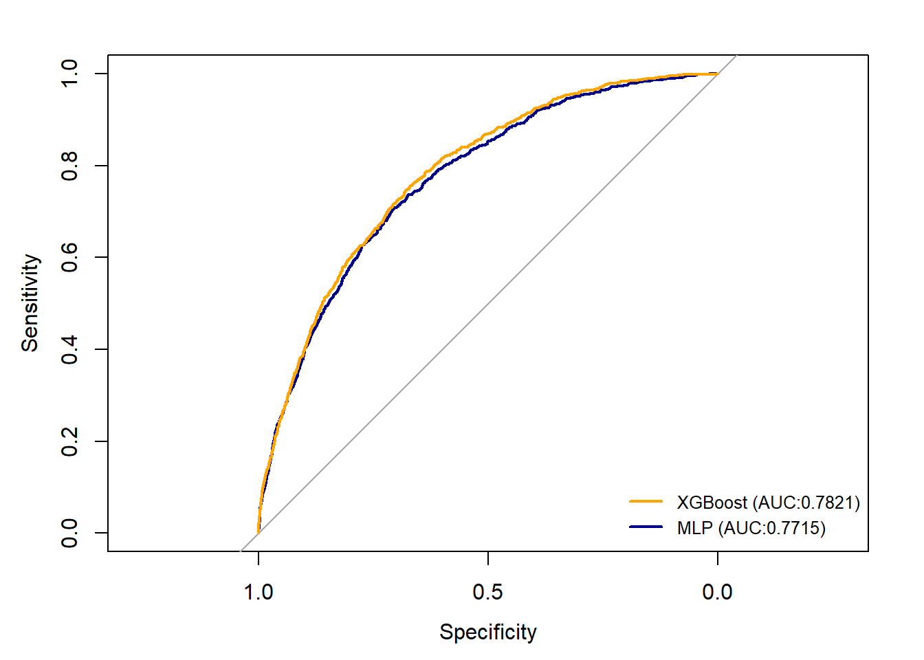
According to the confusion Matrix presented above, we found that the two models have similar performance. XGBoost model has a slightly higher overall accuracy (79%) and MLP model predict better for death_30 cases (69%). Both two models have a Balanced Accuracy at around 70%. Then we plotted Receiver Operating Characteristic (ROC) curves, which also suggests that two models have similar prediction pattern and AUC value.

rocmlp<-roc(controls = results2[data.test.y==0],
            cases = results2[data.test.y==1],
            quiet = TRUE)
rocxgs<-roc(controls = xgbpred[data.test.y==0],
            cases = xgbpred[data.test.y==1],
            quiet = TRUE)

plot(rocmlp, col = "dark blue", lty=1, lwd=2)
plot(rocxgs, add = TRUE,col = "orange", lty=1, lwd=2)
legend("bottomright", legend=c("XGBoost (AUC:0.7821)",
                              "MLP (AUC:0.7715)"),
       col=c("orange", "dark blue"),
       lty=1, lwd=2, cex=0.8, bty="n")